Class 10 Polynomials Notes with Solved Examples
Class 10 Polynomials Notes are essential for mastering algebra and understanding the structure of mathematical expressions. These notes cover key topics such as factorization, the degree of polynomials, zeros of polynomials, remainder, and factor theorems, and solving polynomial equations. Each concept is explained with solved examples and practical problems to help students apply formulas and improve accuracy. By practicing these notes, students can easily learn methods to factorize polynomials, find roots, and solve equations efficiently. Go through the NCERT textbook and solve the NCERT questions with the help of the NCERT Solutions for class 10 Math.s These notes also include tips for solving questions quickly in exams. Polynomials are the basis for quadratic equations, algebraic identities, and higher-level mathematics. Therefore, a strong grasp of polynomial concepts is vital for academic success. These notes are ideal for Class 10 students seeking structured learning material for revision and exam preparation.
What Are Polynomials and Why Do They Matter?
A polynomial is an algebraic expression of the form f(x) = a₀ + a₁x + a₂x² + ... + aₙxⁿ, where a₀, a₁, a₂, ..., aₙ are real numbers and all indices of x are non-negative integers. The highest index n (where aₙ ≠ 0) determines the degree of the polynomial. These mathematical constructs are fundamental to algebra and appear throughout higher mathematics, physics, engineering, and computer science. Understanding polynomials enables students to model real-world phenomena, solve optimization problems, and develop critical analytical thinking skills.
Classification of Polynomials by Degree
Polynomials are categorized based on their degree. A zero-degree polynomial is any non-zero constant (e.g., f(x) = 7), also called a constant polynomial. A linear polynomial has degree 1, taking the form f(x) = ax + b where a ≠ 0, and its graph is always a straight line. A quadratic polynomial has degree 2, expressed as f(x) = ax² + bx + c where a ≠ 0, and its graph forms a parabola. Cubic polynomials have degree 3 and can be written as f(x) = ax³ + bx² + cx + d where a ≠ 0. The degree directly determines the maximum number of zeros (roots) the polynomial can have and the general shape of its graph.
Zeros of Polynomials: Where Functions Cross the X-Axis
A real number α is called a zero of polynomial f(x) if f(α) = 0. Geometrically, zeros represent the points where the graph of the polynomial intersects or touches the x-axis. For a linear polynomial ax + b, the zero is -b/a. A quadratic polynomial can have zero, one, or two real zeros depending on its discriminant D = b² - 4ac. When D > 0, the parabola cuts the x-axis at two distinct points; when D = 0, it touches the x-axis at exactly one point (the vertex); when D < 0, the parabola does not intersect the x-axis and has no real zeros. A cubic polynomial always crosses the x-axis at least once and can have up to three real zeros. Understanding zeros is crucial for solving equations and analyzing function behavior.
Relationship Between Zeros and Coefficients
For a quadratic polynomial f(x) = ax² + bx + c with zeros α and β, two fundamental relationships exist: the sum of zeros equals -b/a (α + β = -b/a) and the product of zeros equals c/a (αβ = c/a). These relationships allow us to construct polynomials from given zeros or to find zeros when coefficients are known. For a cubic polynomial f(x) = ax³ + bx² + cx + d with zeros α, β, and γ, three relationships hold: the sum of zeros equals -b/a (α + β + γ = -b/a), the sum of products taken two at a time equals c/a (αβ + βγ + γα = c/a), and the product of all zeros equals -d/a (αβγ = -d/a). These formulas are derived using the factor theorem and provide powerful tools for polynomial analysis.
Graphing Polynomials: Visual Understanding
The graph of a linear polynomial y = ax + b is a straight line that crosses the x-axis at exactly one point: (-b/a, 0). The graph of a quadratic polynomial y = ax² + bx + c is a parabola. When a > 0, the parabola opens upward; when a < 0, it opens downward. The vertex (turning point) of the parabola is located at (-b/2a, -D/4a) where D = b² - 4ac is the discriminant. By completing the square, any quadratic can be rewritten in the form 4a(y + D/4a) = (2ax + b)², which clearly shows the parabolic nature. The graph of a cubic polynomial has no fixed standard shape but always crosses the x-axis at least once and can have up to two turning points (local maximum and minimum). Drawing polynomial graphs involves creating a table of x and y values, plotting these points, and drawing a smooth curve through them.
Division Algorithm for Polynomials
The division algorithm states that for polynomials p(x) and g(x) with degrees n and m respectively (where m ≤ n), there exist unique polynomials q(x) (quotient) and r(x) (remainder) such that p(x) = q(x) × g(x) + r(x), where r(x) is either zero or has degree less than g(x). This fundamental theorem enables polynomial division similar to arithmetic division. The Remainder Theorem is a special case: when polynomial p(x) is divided by (x - a), the remainder equals p(a). The Factor Theorem extends this: (x - a) is a factor of p(x) if and only if p(a) = 0. These theorems provide efficient methods for finding zeros, factoring polynomials, and solving polynomial equations without performing complete long division.
Essential Polynomial Formulas Reference
| Formula Name | Mathematical Expression | Explanation |
| Quadratic Polynomial | f(x) = ax² + bx + c (a ≠ 0) | Standard form of degree-2 polynomial |
| Cubic Polynomial | f(x) = ax³ + bx² + cx + d (a ≠ 0) | Standard form of degree-3 polynomial |
| Discriminant | D = b² - 4ac | Determines number of real zeros for quadratic |
| Quadratic Vertex | (-b/2a, -D/4a) | Turning point coordinates of parabola |
| Sum of Quadratic Zeros | α + β = -b/a | Relationship for quadratic coefficients |
| Product of Quadratic Zeros | αβ = c/a | Relationship for quadratic coefficients |
| Sum of Cubic Zeros | α + β + γ = -b/a | Relationship for cubic coefficients |
| Sum of Products (Cubic) | αβ + βγ + γα = c/a | Pairwise product relationship for cubic |
| Product of Cubic Zeros | αβγ = -d/a | Relationship for cubic coefficients |
| Quadratic from Zeros | f(x) = k[x² - (α+β)x + αβ] | Construct polynomial from known zeros |
| Division Algorithm | p(x) = q(x)·g(x) + r(x) | Polynomial division relationship |
| Remainder Theorem | p(a) = remainder | When p(x) divided by (x-a) |
| Zero of Linear Polynomial | x = -b/a | For f(x) = ax + b |
Practical Applications and Problem-Solving Strategies
When working with polynomials, several systematic approaches prove valuable. To find zeros of a quadratic, use factoring when possible, apply the quadratic formula x = [-b ± √(b²-4ac)]/(2a), or complete the square. For cubics and higher-degree polynomials, use the Factor Theorem to test potential rational zeros (factors of the constant term divided by factors of the leading coefficient), then apply polynomial division to reduce the degree. When constructing a polynomial from given zeros, multiply the factors (x - α)(x - β)... and expand, or use the sum and product relationships directly. For graphing, always identify the degree (determines basic shape), find zeros and y-intercept, calculate the vertex for quadratics, create a value table, and draw a smooth curve. The discriminant provides quick information about graph behavior without complete plotting.
Common Challenges and How to Overcome Them
Students often struggle with determining when to use which formula. Remember: the discriminant immediately tells you about zeros before solving; zero-coefficient relationships provide quick checks of your solutions; and the factor theorem offers shortcuts for testing potential zeros. When dividing polynomials, organize your work carefully and verify results using the division algorithm equation. For graphing, don't rely on just two or three points—plot sufficient points on both sides of turning points to capture the polynomial's behavior accurately. Understanding that parabolas are symmetric about their axis and that cubic functions have rotational symmetry about inflection points helps sketch more accurate graphs. Always verify your zeros by substituting back into the original polynomial.
This comprehensive understanding of polynomials forms the foundation for advanced mathematics including calculus, differential equations, and abstract algebra. Mastery requires practice with diverse problem types and careful attention to the relationships between algebraic properties and geometric representations.
Find Class 10 Polynomials Notes, Solved Examples & Questions
Polynomials
An algebraic expression f(x) of the form f(x) = a0 + a1x + a2x2 + ...... + anxn where a0, a1, a2, ..., an are real numbers and all the index of x are non-negative integers is called polynomials in x and the highest index n in x is called the degree of the polynomial, if an ≠ 0.
Degree of a Polynomials
(a) Zero Degree Polynomial:
Any non-zero number is regarded as a polynomial of degree zero or zero degree polynomial. For example, f(x) = a, where a ≠ 0 is a zero degree polynomial, since we can write f(x) = a as f(x) = a x0.
(b) Constant Polynomial:
A polynomial of degree zero is called a constant polynomial, e.g. f(x) = 7.
(c) Linear Polynomial:
A polynomial of degree 1 is called a linear polynomial.
e.g. p(x) = 4x - 3 and f(t) = √5t + 5 are linear polynomials.
(d) Quadratic Polynomial:
A polynomial of degree 2 is called a quadratic polynomial.
e.g. f(x) = 2x2 + 5x - 3/5 and g(y) = 3y2 - 5 are quadratic polynomials with real coefficients.
Value of a Polynomial
If f(x) is a polynomial and α is any real number, then the real number obtained by replacing x by α in f(x) is called the value of f(x) at x = α and is denoted by f(α).
e.g. Value of p(x) = 5x2 - 3x + 7 at x = 1 will be:
p(1) = 5(1)2 - 3(1) + 7
= 5 - 3 + 7 = 9
Zeros of a polynomial
A real number α is a zero of polynomial f(x) if f(α) = 0.
The zero of a linear polynomial ax + b is -b/a, i.e. Constant term / Coefficient of x.
Geometrically zero of a polynomial is the point where the graph of the function cuts or touches x-axis.
When the graph of the polynomial does not meet the x-axis at all, the polynomial has no real zero.
Graph of Polynomials - Notes
Graph of Polynomials:
In algebraic or in set theoretic language the graph of a polynomial f(x) is the collection (or set) of all points (x, y), where y = f(x). In geometrical or in graphical language the graph of a polynomial f(x) is a smooth free hand curve passing through points (x1, y1), (x2, y2), (x3, y3), ... etc. where y1, y2, y3, ... are the values of the polynomial f(x) at x1, x2, x3, ... respectively. In order to draw the graph of a polynomial f(x), follow the following algorithm.
Algorithm:
- Step I: Find the values y1, y2, ... yn of polynomial f(x) on different points x1, x2, ... xn and prepare a table that gives values of y or f(x) for various values of x.
| x: | x1 | x2 | ... | xn | xn+1 | ... |
|---|---|---|---|---|---|---|
| y = f(x) | y1 = f(x1) | y2 = f(x2) | ... | yn = f(xn) | yn+1 = f(xn+1) | ... |
- Step II: Plot that points (x1, y1), (x2, y2), (x3, y3), ... (xn, yn) on rectangular co-ordinate system. In plotting these points use different scales on the X and Y axes.
- Step III: Draw a free-hand smooth curve passing through points plotted in step 2 to get the graph of the polynomial f(x).
(a) Graph of a Linear Polynomial:
Consider a linear polynomial f(x) = ax + b, a ≠ 0. Graph of y = ax + b is a straight line. That is why f(x) = ax + b is called a linear polynomial. Since two points determine a straight line, so only two points need to be plotted to draw the line y = ax + b.
The line represented by y = ax + b crosses the X-axis at exactly one point, namely (-b/a, 0).
- Draw the graph of the polynomial f(x) = 2x - 5. Also, find the coordinates of the point where it crosses X-axis.
Sol. Let y = 2x - 5.
The following table lists the values of y corresponding to different values of x.
| x | 1 | 4 |
|---|---|---|
| y | -3 | 3 |
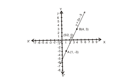
The points A (1, -3) and B (4, 3) are plotted on the graph paper on a suitable scale. A line is drawn passing through these points to obtain the graphs of the given polynomial.
(b) Graph of a Quadratic Polynomial:
Let a, b, c be real numbers and a ≠ 0. Then f(x) = ax2 + bx + c is known as a quadratic polynomial in x. The graph of the quadratic polynomial (i.e. the curve whose equation is y = ax2 + bx + c, a ≠ 0) is always a parabola.
Let y = ax2 + bx + c, where a ≠ 0
⇒ 4ay = 4a x2 + 4abx + 4ac
⇒ 4ay = 4a x2 + 4abx + b2 + 4ac - b2
⇒ 4ay = (2a x + b)2 - (b2 - 4ac)
⇒ 4a y + (b2 - 4ac) = (2a x + b)2
⇒ 4a [ y + (b2 - 4ac)/4a ] = 4a2 [ x + b/(2a) ]2
⇒ y + (b2 - 4ac)/4a = a [ x + b/(2a) ]2
⇒ y + (D/4a) = a (x + b/2a)2 ... (i)
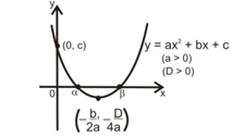
where D = b2 - 4ac is the discriminant of the quadratic equation.
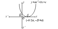
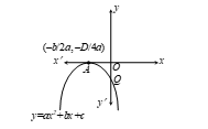
Remarks: Shifting the origin at (-b/2a, -D/4a), we have X = x - (-b/2a) and Y = y - (-D/4a).
Substituting these values in (i), we obtain
Y = aX2 ...(ii) which is the standard equation of a parabola. Clearly, this is the equation of a parabola having its vertex at (-b/2a, -D/4a). The parabola opens upwards or downwards according as a > 0 or a < 0.
SIGNS OF COEFFICIENTS OF A QUADRATIC POLYNOMIAL:
The graphs of y = ax2 + bx + c are given in figure. Identify the signs of a, b and c in each of the following:
- (i) We observe that y = -ax2 + bx + c represents a parabola opening downwards. Therefore, a < 0. We observe that the turning point (-b/2a, -D/4a) of the parabola is in the first quadrant, where D = b2 - 4ac.
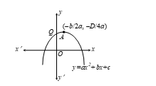
-
∴ -b/2a > 0 ⇒ -b > 0 ⇒ b > 0 in case a < 0
-
Parabola y = ax2 + bx + c cuts y-axis at Q. On y-axis, x = 0.
Putting x = 0 in y = ax2 + bx + c, we get y = c. So, coordinates of Q are (0, c).
As Q lies on the positive direction of y-axis, c > 0.
Hence, a < 0, b > 0, c > 0.
- (ii) We find that y = ax2 + bx + c represents a parabola opening upwards. Therefore, a > 0. The turning point of the parabola is in fourth quadrant.
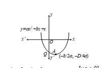
-b/2a > 0 ⇒ -b > 0 ⇒ b > 0. [a > 0]
Parabola y = ax² + bx + c cuts y-axis at Q, x = 0.
Thus, for x = 0 in y = ax² + bx + c, y = c.
Q = (0, c), Q is on negative y-axis, so c < 0.
Hence, a > 0, b > 0, c < 0.
- (iii) Upward Parabola, a > 0, b < 0, c > 0
-b/2a > 0 ⇒ b < 0. [a > 0]
Parabola y = ax² + bx + c has Q on positive y-axis, so c > 0.
Hence, a > 0, b < 0, c > 0.
- (iv) Downward Parabola, a < 0, b < 0, c > 0
Turning point (-b/2a, -D/4a) on negative x-axis.
Hence, a < 0, b < 0, c > 0.
- (v) Upward Parabola, a > 0, b < 0, c > 0, vertex in first quadrant
Turning point (-b/2a, -D/4a) in first quadrant.
-b/2a < 0 ⇒ b < 0. [a > 0]
As Q (0, c) is on positive y-axis, c > 0.
Hence, a > 0, b < 0, c > 0.
- (vi) Downward Parabola, a < 0, b > 0, c < 0
Turning point (-b/2a, -D/4a) in fourth quadrant.
-b/2a > 0 ⇒ b > 0. [a < 0]
Q (0, c) is on negative y-axis, so c < 0.
Hence, a < 0, b > 0, c < 0.
HOW TO DRAW GRAPH OF QUADRATIC POLYNOMIALS
- Write the given quadratic polynomial f(x) = ax2 + bx + c as
y = ax2 + bx + c - Calculate the zeros of the polynomial, if exist, by putting y = 0 i.e., ax2 + bx + c = 0
- Calculate the points where the curve meets y-axis by putting x = 0.
- Calculate D = b2 - 4ac
D > 0, graph cuts x-axis at two points.
D = 0, graph touches x-axis at one point.
D < 0, graph is far away from x-axis. - Find - b / (2a) which is the turning point of curve.
- Make a table of selecting values of x and corresponding values of y, two to three values on left and two to three values on right of turning point
- Draw a smooth curve through these points by free hand. The graph so obtained is called a parabola.
- Draw the graph of the polynomial f(x) = x2 - 2x - 8
Sol. Let y = x2 - 2x - 8.
The following table gives the values of y or f(x) for various values of x.
| x | -4 | -3 | -2 | -1 | 0 | 1 | 2 | 3 | 4 | 5 | 6 |
|---|---|---|---|---|---|---|---|---|---|---|---|
| y = x2 - 2x - 8 | 16 | 7 | 0 | -5 | -8 | -9 | -8 | -5 | 0 | 7 | 16 |
Let us plot the points (-4, 16), (-3, 7), (-2, 0), (-1, -5), (0, -8), (1, -9), (2, -8), (3, -5), (4, 0), (5, 7) and (6, 16) on a graph paper and draw a smooth free hand curve passing through these points. The curve thus obtained represents the graphs of the polynomial f(x) = x2 - 2x - 8. This is called a parabola. The lowest point P, called a minimum point, is the vertex of the parabola. Vertical line passing through P is called the axis of the parabola. Parabola is symmetric about the axis. So, it is also called the line of symmetry.
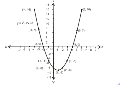
Observations:
- The coefficient of x2 in f(x) = x2 - 2x - 8 is 1 (a positive real number) and so the parabola opens upwards.
- D = b2 - 4ac = 4 + 32 = 36 > 0; so, the parabola cuts X axis at two distinct points.
- On comparing the polynomial x2 - 2x - 8 with ax2 + bx + c, we get a = 1, b = -2 and c = -8. The vertex of the parabola has coordinates (1, -9) i.e. ( -b / 2a, ( -D / 4a) ), where D = b2 - 4ac.
- The polynomial f(x) = x2 - 2x - 8 = (x - 4)(x + 2) is factorizable into two distinct linear factors (x - 4) and (x + 2). So, the parabola cuts X-axis at two distinct points (4, 0) and (-2, 0). The X-coordinates of these points are zeros of f(x).
GRAPH OF A CUBIC POLYNOMIAL
Graphs of a cubic polynomial does not have a fixed standard shape. Cubic polynomial graphs will always cross X-axis at least once and at most thrice.
- Draw the graphs of the polynomial f(x) = x3 - 4x
Sol. Let y = f(x) or y = x3 - 4x
The values of y for variable value of x are listed in the following table:
| x | -3 | -2 | -1 | 0 | 1 | 2 | 3 |
|---|---|---|---|---|---|---|---|
| y = x3 - 4x | -15 | 0 | 3 | 0 | -3 | 0 | 15 |
Thus, the curve y = x3 - 4x passes through the points (-3, -15), (-2, 0), (-1, 3), (0, 0), (1, -3), (2, 0), (3, 15), (4, 48) etc. Plotting these points on a graph paper and drawing a free hand smooth curve through these points, we obtain the graph of the given polynomial as shown figure.
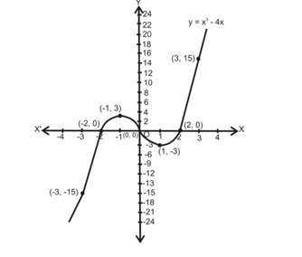
Observations
- The polynomial f(x) = x³ - 4x = x(x² - 4) = x(x - 2)(x + 2) is factorizable into three distinct linear factors. The curve y = f(x) = x³ - 4x also cuts the X-axis at three distinct points.
- We have, f(x) = x(x - 2)(x + 2). Therefore, 0, 2 and -2 are three zeros of f(x). The curve y = f(x) cuts X-axis at three points (0, 0), (2, 0), and (-2, 0).
RELATIONSHIP BETWEEN ZEROS AND COEFFICIENTS OF A QUADRATIC POLYNOMIAL
Let α and β be the zeros of a quadratic polynomial f(x) = ax² + bx + c. By factor theorem, (x – α) and (x – β) are the factors of f(x).
f(x) = k(x – α)(x – β)
ax² + bx + c = k[x² – (α + β)x + αβ]
Comparing the coefficients of x², x, and constant terms on both sides, we get:
a = k
b = –k(α + β)
c = kαβ
α + β = –b/a
αβ = c/a
- Sum of the zeros = –b/a = Coefficient of x / Coefficient of x²
- Product of the zeros = c/a = Constant term / Coefficient of x²
Remarks
If α and β are the zeros of a quadratic polynomial f(x), the polynomial f(x) is given by:
f(x) = k[x² – (Sum of the zeros)x + Product of the zeros]
Example
- Find a quadratic polynomial whose zeros are 5 + √2 and 5 – √2.
Sol. Given α = 5 + √2, β = 5 – √2
f(x) = k[x² – (α + β)x + αβ]
α + β = 10, αβ = (5 + √2)(5 – √2) = 25 – 2 = 23
So, f(x) = k[x² – 10x + 23], where k is any non-zero real number.
RELATIONSHIP BETWEEN ZEROS AND COEFFICIENTS OF A CUBIC POLYNOMIAL
Let α, β, γ be the zeros of a cubic polynomial f(x) = ax³ + bx² + cx + d, a ≠ 0. By factor theorem, (x – α), (x – β) and (x – γ) are factors of f(x). Also, f(x) (being cubic) cannot have more than three linear factors.
f(x) = k(x – α)(x – β)(x – γ)
ax³ + bx² + cx + d = k[x³ – (α + β + γ)x² + (αβ + βγ + γα)x – αβγ]
Comparing coefficients on both sides, we get:
a = k
b = –k(α + β + γ)
c = k(αβ + βγ + γα)
d = –k(αβγ)
α + β + γ = –b/a
αβ + βγ + γα = c/a
αβγ = –d/a
- Sum of the zeros = –b/a = Coefficient of x² / Coefficient of x³
- Sum of products of zeros two at a time = c/a = Coefficient of x / Coefficient of x³
- Product of the zeros = –d/a = Constant term / Coefficient of x³
Remarks
Cubic polynomial having zeros α, β and γ is given by:
f(x) = k(x – α)(x – β)(x – γ)
or f(x) = k[x³ – (α + β + γ)x² + (αβ + βγ + γα)x – αβγ], where k is any non-zero real number.
Example
- Form a cubic polynomial with zeros α = 3, β = 2, γ = –1.
Sol. α = 3, β = 2, γ = –1
Required polynomial = k[(x – 3)(x – 2)(x + 1)]
= k[x³ – 5x² + 5x + 6]
Division Algorithm and Theorems for Polynomials
Let p(x) and g(x) be polynomials of degree n and m respectively such that m ≤ n. Then there exist unique polynomials q(x) and r(x) where r(x) is either zero polynomial or degree of r(x) < degree of g(x) such that p(x) = g(x) · q(x) + r(x).
p(x) is dividend, g(x) is divisor.
q(x) is quotient, r(x) is remainder.
FACTOR THEOREM
Let p(x) be a polynomial of degree greater than or equal to 1 and ‘a’ be a real number such that p(a) = 0. Then (x - a) is a factor of p(x). Conversely, if (x - a) is a factor of p(x), then p(a) = 0.
- Show that x + 1 and 2x - 3 are factors of 2x³ - 9x² + x + 12.
Sol. To prove that (x + 1) and (2x - 3) are factors of p(x) = 2x³ - 9x² + x + 12 it is sufficient to show that p(-1) and p(3/2) both are equal to zero.
p(-1) = 2(-1)³ – 9(-1)² + (-1) + 12 = -2 – 9 + (-1) + 12 = -2 – 9 -1 +12 = -12 +12 = 0
And
p(3/2) = 2(3/2)³ – 9(3/2)² + (3/2) + 12
= 2·27/8 – 9·9/4 + 3/2 + 12
= 27/4 – 81/4 + 3/2 + 12
= 27 – 81 + 6 + 48/4
= -81 + 81/4 = 0
REMAINDER THEOREM
Let p(x) be any polynomial of degree greater than or equal to one and ‘a’ be any real number. If p(x) is divided by (x – a), then the remainder is equal to p(a).
Let q(x) be the quotient and r(x) be the remainder when p(x) is divided by (x – a), then:
Dividend = Divisor × Quotient + Remainder
- Find the remainder when f(x) = x³ – 6x² + 2x – 4 is divided by g(x) = 1 – 2x.
Sol. 1 – 2x = 0 ⇒ 2x = 1 ⇒ x = 1/2.
f(1/2) = (1/2)³ – 6 × (1/2)² + 2 × (1/2) – 4
= 1/8 – 6/4 + 1 – 4
= 1/8 – 3/2 + 1 – 4
= 1/8 – 12/8 + 8/8 – 32/8
= (1 – 12 + 8 – 32)/8
= –35/8 - Apply division algorithm to find the quotient q(x) and remainder r(x) on dividing f(x) = 10x⁴ + 17x³ - 62x² + 30x - 3 by g(x) = 2x² + x + 1.
Sol. 5x² + 11x + 28
2x² - x + 1 ) 10x⁴ + 17x³ – 62x² + 30x – 3
(Steps of polynomial division moving through all columns as in the original image)
So, quotient q(x) = 5x² + 11x + 28 and remainder r(x) = –9x + 25.
Now, dividend = Divisor × Quotient + Remainder
= (5x² + 11x + 28)(2x² + x + 1) + (–9x + 25)
= 10x⁴ + 17x³ – 62x² + 30x – 3
Hence, the division algorithm is verified.
Questions:
- Find a quadratic polynomial whose zeros are 2 and –3.
- Find the polynomial p(x) whose graph is given below:
- Draw the graph of the polynomial f(x) = x² + 2x – 3.
- Find a quadratic polynomial whose zeros are reciprocals of the zeros of the polynomial f(x) = ax² + bx + c, a ≠ 0, c ≠ 0.
- Sum of product of zeros of quadratic polynomial are 5 and 17 respectively. Find the polynomial.
- Show that x = 2 is a root of 2x² + x² – 7x – 6.
Answers:
- 1. k
- 2. g(x) = k(x² – 5x + P) = k[x² + (b/c)x + a/c]
- 5. k(x² – 5x + 17)
1. Find a quadratic polynomial whose zeros are 2 and –3.
Sol.
Required polynomial is:
k(x – 2)[x – (–3)]
= k(x – 2)(x + 3)
= k(x² + x – 6)
where k is a non-zero constant.
2. Find the polynomial p(x) whose graph is given below:
(X-intercepts: –1, 0 and 4, 0; vertex at 0, 3)
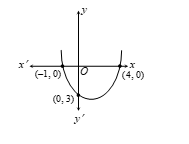
Sol. As the parabola intersects x-axis at 4 and -1,
Required polynomial is:
k[(x + 1)(x - 4)]
= k(x2 - 4x + x - 4)
= k(x2 - 3x - 4)
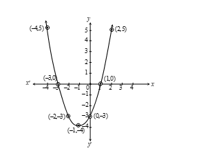
3. Draw the graph of the polynomial f(x) = x2 + 2x - 3.
Sol.
Let y = x2 + 2x - 3 is the given polynomial.
Since the coefficient of x2 is positive, it will open upward.
a = 1, b = 2, c = -3
D = b2 - 4ac = (2)2 - 4×1×-3 = 4 + 12 = 16
As D > 0, so parabola cuts x-axis at two points.
If y = 0:
x2 + 2x - 3 = 0
x2 + 3x - x - 3 = 0
x(x + 3) - 1(x + 3) = 0
(x - 1)(x + 3) = 0
x = 1 or x = -3
It shows the graph of f(x) will intersect x-axis at (1, 0) and (-3, 0).
Vertex = \( \left( -\frac{b}{2a}, -\frac{D}{4a} \right) = \left( -\frac{2}{2}, -\frac{16}{4} \right) = (-1, -4) \)
Required table:
| x | -4 | -3 | -2 | -1 | 0 | 2 |
|---|---|---|---|---|---|---|
| x2 | 16 | 9 | 4 | 1 | 0 | 4 |
| +2x | -8 | -6 | -4 | -2 | 0 | 4 |
| y = x2 + 2x - 3 | 5 | 0 | -3 | -4 | -3 | 5 |
4. Find a quadratic polynomial whose zeros are reciprocals of the zeros of given f(x) = ax2 + bx + c, a ≠ 0, c ≠ 0.
Sol.
Let α, β be the zeros of f(x).
α + β = -b/a and αβ = c/a
New zeros = 1/α, 1/β
Let S and P be the sum and product:
S = 1/α + 1/β = (α + β) / (αβ) = (-b/a) / (c/a) = -b/c
P = (1/α)·(1/β) = 1/(αβ) = a/c
Required polynomial:
g(x) = k[x2 + Sx + P] = k\left[ x2 + \frac{b}{c}x + \frac{a}{c} \right]
where k is any non-zero constant.
5. Sum and product of zeros of quadratic polynomial are 5 and 17 respectively. Find the polynomial.
Sol.
Given: Sum of zeros = 5
Product = 17
Required polynomial:
f(x) = k\left[ x^2 - 5x + 17 \right], \text{ where k is any non-zero real number.}
6. Show that x = 2 is a root of 2x2 + x2 – 7x – 6.
Sol.
f(x) = 2x2 + x2 – 7x – 6
f(2) = 2(2)2 + (2)2 – 7·2 – 6
= 2·4 + 4 – 14 – 6
= 8 + 4 – 14 – 6
= 12 – 20 = –8
Since this does not equal zero, please verify the original expression.
Questions:
- Find α and β if x + 1 and x + 2 are factors of p(x) = x3 + 3x2 - 2αx + β.
- What must be added to 3x3 + x2 - 22x + 9 so that the result is exactly divisible by 3x2 + 7x - 6.
- Find the value for K for which x4 + 10x3 + 25x2 + 15x + K exactly divisible by x + 7.
- Find the Quadratic polynomial whose sum and product of zeros are \(\sqrt{2} + 1\), \(1/\sqrt{2} + 1\).
- If (n-k) is a factor of the polynomials x2 + px + q & x2 + mx + n, prove that k = n + (n-q)/(m-p).
Answers:
7. α = –1, β = 0
8. 2x + 3, 9, 91
7. Find α and β if x + 1 and x + 2 are factors of p(x) = x3 + 3x2 - 2αx + β.
Sol.
x + 1 and x + 2 are factors.
Then, p(-1) = 0 and p(-2) = 0
p(-1) = (-1)3 + 3(-1)2 - 2α(-1) + β = –1 + 3 – 2α(-1) + β = 0
⇒ –1 + 3 + 2α + β = 0 ⇒ 2α + β = –2 ... (i)
p(-2) = (–2)3 + 3(–2)2 – 2α(–2) + β = –8 + 12 + 4α + β = 0
⇒ 4α + β = –4 ... (ii)
Subtract (i) from (ii):
(4α + β) – (2α + β) = –4 – (–2)
2α = –4 + 2 = –2
⇒ α = –1
Now, from (i), 2α + β = –2, so 2(–1) + β = –2
β = 0
Hence α = –1, β = 0
8. What must be added to 3x3 + x2 – 22x + 9 so that the result is exactly divisible by 3x2 + 7x – 6
Sol.
Let p(x) = 3x3 + x2 – 22x + 9 and q(x) = 3x2 + 7x – 6.
We know if p(x) is divided by q(x), remainder should be 0.
Suppose we add 2x + 3: p(x) + 2x + 3 = 3x3 + x2 – 22x + 9 + 2x + 3 = 3x3 + x2 – 20x + 12
Now, using division:
3x3 + x2 – 20x + 12 ÷ 3x2 + 7x – 6
–> (Detailed calculation, long division steps; see original for full working)
The remainder is zero when
a = –2, b = –3
Therefore 2x + 3 must be added.
9. Find the value for K for which x4 + 10x3 + 25x2 + 15x + K exactly divisible by x + 7
Sol.
Let P(x) = x4 + 10x3 + 25x2 + 15x + K, g(x) = x + 7.
Divide P(x) by g(x).
As the remainder must be zero,
Substitute x = –7 in P(x) and set P(–7) = 0.
P(–7) = (–7)4 + 10(–7)3 + 25(–7)2 + 15(–7) + K = 2401 – 3430 + 1225 – 105 + K = 91 + K
91 + K = 0 ⇒ K = –91
10. Find the Quadratic polynomial whose sum and product of zeros are √2 + 1, 1/(√2 + 1)
Sol.
sum = √2 + 1
product = 1 / (√2 + 1)
Required polynomial is:
x2 – (sum)x + product
= x2 – (√2 + 1)x + 1/(√2 + 1)
11. If (n – k) is a factor of the polynomials x2 + px + q and x2 + mx + n, prove that k = n + (n – q)/(m – p)
Sol. Given (n – k) is a factor of both:
So (n – k)2 + p(n – k) + q = 0
And (n – k)2 + m(n – k) + n = 0
Subtract second from first:
[p – m](n – k) + q – n = 0
n – k = (n – q)/(m – p)
k = n + (n – q)/(m – p)