Detailed Class 10 Statistics Notes with Graphical Examples
Class 10 Statistics Notes cover the key concepts of mean, median, mode, cumulative frequency, and graphical representation of data. These notes explain each topic with solved examples, practical exercises, and stepwise methods for accurate calculations. Understanding statistics is crucial for data interpretation, problem-solving, and real-life applications. The notes include tips and shortcuts for calculating statistical measures quickly and efficiently. With practice problems and revision strategies, students can improve accuracy, speed, and conceptual clarity. These notes are ideal for Class 10 students preparing for board exams and competitive tests, helping them confidently tackle questions related to statistics. Students must solve the NCERT questions with the help of the NCERT Solutions for class 10 Maths, which will help in building the foundation.
Class 10 Statistics Notes, Solved example & Questions
Introduction
Suppose we want to compare the income distribution of workers in two factories and determine which factory pays more to its workers. If we compare on the basis of individual workers, we cannot conclude anything. However, if for the given data, we get a representative value that signifies the characteristics of the data, the comparison becomes easy.
It is generally observed that observations or data on a variable tend to gather around some central value. This gathering of data towards a central value is called central tendency or the middle value of the distribution, also known as middle of the data set.
Measures of Central Tendency
The commonly used measure of central tendency (or averages) are:
- (i) Arithmetic Mean (AM) or Simply Mean
- (ii) Median
- (iii) Mode
Arithmetic Mean
Arithmetic mean is a set of observations that is equal to their sum divided by the total number of observations. Mean is denoted by x̄.
Mean of Raw Data
If x₁, x₂, x₃, ....., xₙ are the n values (or observations) then,
x̄ = (x₁ + x₂ + ..... + xₙ)/n = (Σxᵢ)/n
nx̄ = Sum of observations = Σxᵢ
i.e. product of mean & no. of items gives sum of observation.
Example 1:
Problem: The mean of marks scored by 100 students was found to be 40. Later on it was discovered that a score of 56 was misread as 83. Find the correct mean.
Solution:
n = 100, x̄ = 40
x̄ = (1/n)(Σxᵢ) ⇒ 40 = (1/100)(Σxᵢ)
∴ Incorrect value of Σxᵢ = 4000
Now, Correct value of Σxᵢ = 4000 - 83 + 56 = 3973
Correct mean = (correct value of Σxᵢ)/n = 3973/100 = 39.73
Answer: The correct mean is 39.73
Method for Mean of Ungrouped Data
| xᵢ | fᵢ | fᵢxᵢ |
|---|---|---|
| x₁ | f₁ | f₁x₁ |
| x₂ | f₂ | f₂x₂ |
| x₃ | f₃ | f₃x₃ |
| ... | ... | ... |
| Σfᵢ | Σfᵢxᵢ |
Mean for a Group Frequency Distribution
DIRECT METHOD:
Step 1: For each class, find the class mark xᵢ as
Step 2: Calculate fᵢxᵢ for each i.
Step 3: Use the formula:
Example 1:
Problem: Find the arithmetic mean of 1, 2, 3, …., n.
Solution:
The arithmetic mean of 1, 2, 3, ….., n is given by
x̄ = (1 + 2 + 3 + .... + n)/n
= (n/2)[2×1 + (n-1)×1]/n
= (n+1)/2
Example 2:
Problem: If the mean of n observations is X̄, then find the new mean when the first term is increased by 1, second term by 2, and so on.
Solution:
X̄ = (x₁ + x₂ + .... + xₙ)/n = Σxᵢ/n
new mean = [(x₁+1) + (x₂+2) + (x₃+3) + .... + (xₙ+n)]/n
= [(x₁ + x₂ + x₃ + ..... + xₙ) + (1+2+3+ .... +n)]/n
= Σxᵢ/n + (1+2+3+....+n)/n
= X̄ + (n/2)[2×1+(n-1)×1]/n
= X̄ + (n+1)/2
Assumed Mean Method
Following steps are taken to solve cases by assumed-mean method:
Step 1: For each class interval, calculate the class mark xᵢ by using the formula:
Step 2: Choose a value of xᵢ in the middle as the assumed mean and denote it by A.
Step 3: Calculate the deviations dᵢ = (xᵢ - A) for each i.
Step 4: Calculate the (fᵢdᵢ) for each i.
Step 5: Find n = Σfᵢ.
Step 6: Calculate the mean, x̄, by using the formula:
Example 1:
Problem: Using the assumed-mean method, find the mean of the following data:
| Class | 0-10 | 10-20 | 20-30 | 30-40 | 40-50 |
|---|---|---|---|---|---|
| Frequency | 7 | 8 | 12 | 13 | 10 |
Solution: Let A = 25 be the assumed mean. Then, we have:
| Class interval | Frequency fᵢ | Midvalue xᵢ | Deviation dᵢ = (xᵢ - 25) | (fᵢdᵢ) |
|---|---|---|---|---|
| 0-10 | 7 | 5 | -20 | -140 |
| 10-20 | 8 | 15 | -10 | -80 |
| 20-30 | 12 | 25 = A | 0 | 0 |
| 30-40 | 13 | 35 | 10 | 130 |
| 40-50 | 10 | 45 | 20 | 200 |
| Σfᵢ = 50 | Σ(fᵢdᵢ) = 110 |
∴ x̄ = A + Σfᵢdᵢ/n = 25 + 110/50 = 25 + 2.2 = 27.2
Answer: Hence, mean = 27.2
Step-Deviation Method
Following steps are taken to solve cases by step-deviation method:
Step 1: For each class interval, calculate the class mark xᵢ by using the formula:
Step 2: Choose a value of xᵢ in the middle of the xᵢ column as the assumed mean and denote it by A.
Step 3: Calculate h = [(upper limit) – (lower limit)].
Step 4: Calculate uᵢ = (xᵢ - A)/h for each class.
Step 5: Calculate fᵢuᵢ for each class and find Σ(fᵢuᵢ).
Step 6: Calculate the mean, by using the formula:
Example 1:
Problem: Calculate the mean of the following frequency distribution, using the step-deviation method:
| Class interval | Frequency |
|---|---|
| 0-50 | 17 |
| 50-100 | 35 |
| 100-150 | 43 |
| 150-200 | 40 |
| 200-250 | 21 |
| 250-300 | 24 |
Solution: Here, h = 50. Let the assumed mean be A = 125.
For calculating the mean, table is prepared as follows:
| Class interval | Frequency fᵢ | Midvalue xᵢ | uᵢ = (xᵢ - A)/h | (fᵢuᵢ) |
|---|---|---|---|---|
| 0-50 | 17 | 25 | -2 | -34 |
| 50-100 | 35 | 75 | -1 | -35 |
| 100-150 | 43 | 125 = A | 0 | 0 |
| 150-200 | 40 | 175 | 1 | 40 |
| 200-250 | 21 | 225 | 2 | 42 |
| 250-300 | 24 | 275 | 3 | 72 |
| Σfᵢ = 180 | Σ(fᵢuᵢ) = (154-69) = 85 |
Thus, we have A = 125, h = 50, Σfᵢ = 180 and Σ(fᵢuᵢ) = 85.
Mean, x̄ = A + h[Σ(fᵢuᵢ)/Σfᵢ]
= 125 + 50×(85/180)
= (125 + 23.61) = 148.61
Answer: Hence, the mean of the given frequency is 148.61
Properties of Mean
- (i) Sum of deviations from mean is zero. i.e. Σ(xᵢ - x̄) = 0
- (ii) If a constant real number 'a' is added to each of the observation then new mean will be x̄ + a.
- (iii) If a constant real number 'a' is subtracted from each of the observation then new mean will be x̄ - a.
- (iv) If constant real number 'a' is multiplied with each of the observation then new mean will be ax̄.
- (v) If each of the observation is divided by a constant no 'a', then new mean will be x̄/a.
Merita and Demerits of Arithmetic Mean
Merits of Arithmetic Mean:
- (i) It is rigidly defined, simple, easy to understand and easy to calculate.
- (ii) It is based upon all the observations.
- (iii) Its value being unique, we can use it to compare different sets of data.
- (iv) It is least affected by sampling fluctuations.
- (v) Mathematical analysis of mean is possible. So, It is relatively reliable.
Demerits of Arithmetic Mean:
- (i) It cannot be determined by inspection nor it can be located graphically.
- (ii) Arithmetic mean cannot be used for qualities characteristics such as intelligence, honesty, beauty etc.
- (iii) It cannot be obtained if a single observation is missing.
- (iv) It is affected very much by extreme values. In case of extreme items, A.M. gives a distorted picture of the distribution and no longer remains representative of the distribution.
- (v) It may lead to wrong conclusions if the details of the data from which it is computed are not given.
- (vi) It cannot be calculated if the extreme class is open, e.g. below 10 or above 90.
- (vii) It cannot be used in the study of ratios, rates etc.
Uuse of Arithmetic Mean:
- (i) It is used for calculating average marks obtained by a student.
- (ii) It is extensively used in practical statistics and to obtain estimates.
- (iii) It is used by businessman to find out profit per unit article, output per machine, average monthly income and expenditure etc.
Median
Median is the middle value of the distribution. It is the value of variable such that the number of observations above it is equal to the number of observations below it.
Median of Raw Data:
(i) Arrange the data in ascending order.
(ii) Count the no. of observation (Let there be 'n' observation)
(B) If n is even then median is the arithmetic mean of [n/2]th observation and [n/2 + 1]th observation.
Example 1:
Problem: Following are the lives in hours of 15 pieces of the components of aircraft engine. Find the median:
715, 724, 725, 710, 729, 745, 649, 699, 696, 712, 734, 728, 716, 705, 719
Solution: Arranging the data in ascending order
649, 696, 705, 710, 712, 715, 716, 719, 724, 725, 728, 729, 734, 745
N = 15
So, Median = [(N+1)/2]th observation
= [(15+1)/2]th observation
= 8th observation
= 716
Median of Class-Interval Data (Grouped)
Where:
ℓ = lower limit of median class
N = total no of observation
C = cumulative frequency of the class preceding the median class
h = size of the median class
f = frequency of the median class
What is median class: The class in which [N/2]th item lie is median class.
Example 1:
Problem: The daily wages (in rupees) of 100 workers in a factory are given below. Find the median wage of a worker for the above date.
| Daily wages (in Rs.) | 125 | 130 | 135 | 140 | 145 | 150 | 160 | 180 |
|---|---|---|---|---|---|---|---|---|
| No. of workers | 6 | 20 | 24 | 28 | 15 | 4 | 2 | 1 |
Solution:
| Daily wages (in Rs.) | No. of workers | Cumulative frequency |
|---|---|---|
| 125 | 6 | 6 |
| 130 | 20 | 26 |
| 135 | 24 | 50 |
| 140 | 28 | 78 |
| 145 | 15 | 93 |
| 150 | 4 | 97 |
| 160 | 2 | 99 |
| 180 | 1 | 100 |
N = 100 (even)
∴ Median = [50th observation + 51st observation]/2
Median = (135 + 140)/2 = 137.50
Answer: Median wage of workers in the factory is Rs 137.50
Merits and Demerits of Median
Merits of Median:
- (i) It is rigidly defined, easily, understood and calculate.
- (ii) It is not all affected by extreme values.
- (iii) It can be located graphically, even if the class-intervals are unequal.
- (iv) It can be determined even by inspection is some cases.
Demerits of Median:
- (i) In case of even numbers of observations median cannot be determined exactly.
- (ii) It is not based on all the observations.
- (iii) It is not subject to algebraic treatment.
- (iv) It is much affected by fluctuations of sampling.
Uuses od Median:
- (i) Median is the only average to be used while dealing with qualitative data which cannot be measured quantitatively but can be arranged in ascending or descending order of magnitude.
- (ii) It is used for determining the typical value in problems concerning wages, distribution of wealth etc.
Mode
It is that value of a variate which occurs most often. More precisely, mode is that value of the variable at which the concentration of the data is maximum.
Modal Class: In a frequency distribution, the class having maximum frequency is called the modal class.
Example 1:
Problem: The wickets taken by a bowler in 10 cricket matches are as follows: 2, 6, 4, 5, 0, 2,1, 3, 2, 3. Find the mode of the data.
Solution: Clearly, 2 is the number of wickets taken by the bowler in the maximum number (i.e., 3) of matches. So, the mode of the distribution is 2.
Formula for Calculating Mode:
where:
ℓ = lower limit of the modal class
f₁ = frequency of the modal class
f₀ = frequency of the class preceding the modal class
f₂ = frequency of the class succeeding the modal class
h = width of the class interval (assuming all class width to be equal)
Example 2:
Problem: For what value of x, the mode of the following data is 7: 3, 5, 6, 7, 5, 4, 7, 5, 6, x, 8, 7.
Solution:
| Variate | 3 | 4 | 5 | 6 | 7 | 8 |
|---|---|---|---|---|---|---|
| Frequency | 1 | 1 | 3 | 2 | 3 | 1 |
5 and 7 both have maximum frequency, but mode = 7. So, x = 7.
Merits and Demerits of Mode
Merits of Mode:
- (i) It can be easily understood and is easy to calculate.
- (ii) It is not affected by extreme values and can be found by inspection is some cases.
- (iii) It can be measured even if open-end classes and can be represented graphically.
Demerits and Mode:
- (i) It is ill-defined. It is not always possible to find a clearly defined mode.
- (ii) It is not based upon all the observation.
- (iii) It is not capable of further mathematical treatment. It is after indeterminate.
- (iv) It is affected to a greater extent by fluctuations of sampling.
Uses of Mode:
Mode is the average to be used to find the ideal size, e.g., in business forecasting, in manufacture of ready-made garments, shoes etc.
Relationship Among Mean, Median and Mode
or
Median = Mode + (2/3)(Mean - Mode)
or
Mean = Mode + (3/2)(Median - Mode)
Cumulative Frequency Curve or Ogive Graph
In a cumulative frequency polygon or curves, the cumulative frequencies are plotted against the lower and upper limits of class intervals depending upon the manner in which the series has been cumulated. There are two methods of constructing a frequency polygon or an Ogive.
- (i) Less than method
- (ii) More than method
Example 1:
Problem: The marks obtained by 400 students in medical entrance exam are given in the following table.
| Marks Obtained | 400-450 | 450-500 | 500-550 | 550-600 | 600-650 | 650-700 | 700-750 | 750-800 |
|---|---|---|---|---|---|---|---|---|
| No. of Examinees | 30 | 45 | 60 | 52 | 54 | 67 | 45 | 47 |
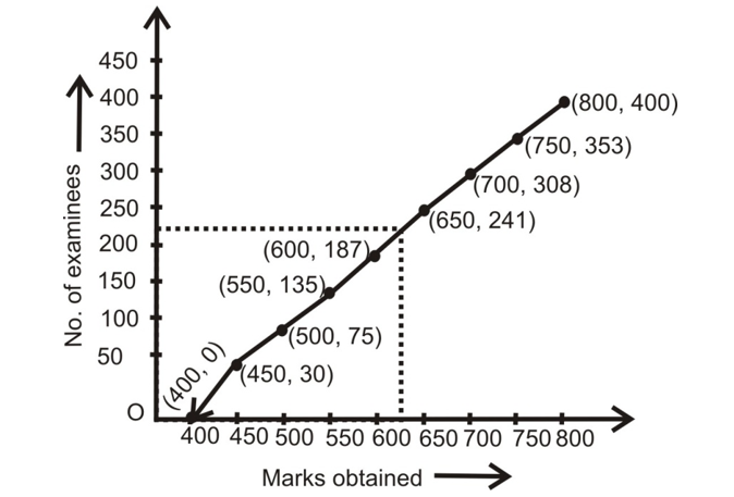
(i) Draw Ogive by less than method.
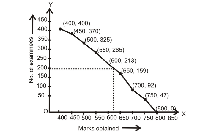
(ii) Draw Ogive by more than method.
(iii) Find the number of examinees, who have obtained the marks less than 625.
(iv) Find the number of examinees, who have obtained 625 and more than marks.
Solution:
(i) Cumulative frequency table for less than Ogive method is as following:
| Marks Obtained | No. of Examinees |
|---|---|
| Less than 450 | 30 |
| Less than 500 | 75 |
| Less than 550 | 135 |
| Less than 600 | 187 |
| Less than 650 | 241 |
| Less than 700 | 308 |
| Less than 750 | 353 |
| Less than 800 | 400 |
Following are the Ogive for the above cumulative frequency table by applying the given method and the assumed scale.
(ii) Cumulative frequency table for more than Ogive method is as following:
| Marks Obtained | No. of Examinees |
|---|---|
| 400 and more | 400 |
| 450 and more | 370 |
| 500 and more | 325 |
| 550 and more | 265 |
| 600 and more | 213 |
| 650 and more | 159 |
| 700 and more | 92 |
| 750 and more | 47 |
(iii) So, the number of examinees, scoring marks less than 625 are approximately 220.
(iv) So, the number of examinees, scoring marks 625 and more will be approximately 190.
Statistics
Summary - Statistics
| Concept | Formula/Description |
|---|---|
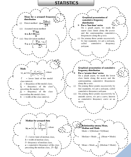
| Mean for grouped frequency distribution | (i) Direct method: x̄ = Σ(fᵢxᵢ)/Σfᵢ (ii) Assumed-mean method: x̄ = A + Σfᵢdᵢ/n (iii) Step-deviation method: x̄ = A + h[Σ(fᵢuᵢ)/Σfᵢ] |
| Mode | M₀ = ℓ + h[(f₁ - f₀)/(2f₁ - f₀ - f₂)] where ℓ = lower limit of the modal class interval f₁ = frequency of the modal class f₀ = frequency of the class preceding the modal class f₂ = frequency of the class succeeding the modal class h = width of the class interval |
| Median for grouped data | Me = ℓ + h[(N/2 - c)/f] where ℓ = lower limit of median class h = width of median class f = frequency of median class c = cumulative frequency of the class preceding the median class N = Σfᵢ |
| Relationship among Mean, Median and Mode | Mode = 3(Median) - 2(Mean) or Median = Mode + (2/3)(Mean - Mode) or Mean = Mode + (3/2)(Median - Mode) |
| Graphical presentation of cumulative frequency distribution | For 'less than' series: On a graph paper, mark the upper class limits along the x-axis and the corresponding cumulative frequencies along the y-axis. (i) On joining these points successively by line segments, we get a polygon, called cumulative frequency polygon. (ii) On joining these points successively by smooth curves, we get a curve, known as cumulative frequency curve or an ogive. For 'greater than' series: On a graph paper, mark the lower class limits along the x-axis and the corresponding cumulative frequencies along the y-axis. (i) On joining these points successively by line segments, we get a polygon, called cumulative frequency polygon. (ii) On joining these points successively by smooth curves, we get a curve, known as cumulative frequency curve or an ogive. |
Pratices Exercises
Note: The PDF contains multiple exercise sets (Exercise 1, 2, 3, and 4) with numerous practice problems. Due to length constraints, I'm including the structure. All exercises contain multiple choice questions and numerical problems covering:
- Calculation of mean using different methods
- Finding median from grouped and ungrouped data
- Determining mode
- Drawing and interpreting ogive curves
- Finding missing frequencies
- Application problems in real-world contexts
Answer Keys
Exercise - 1 Answers:
| 1. (c) | 2. (b) | 3. (b) | 4. (a) | 5. (c) |
| 6. (d) | 7. (b) | 8. (b) | 9. (a) | 10. (c) |
| 11. (b) | 12. (a) | 13. (b) | 14. (b) | 15. (c) |
| 16. (a) | 17. (b) | 18. (c) | 19. (a) | 20. (b) |
| 21. (a) | 22. (b) | 23. (a) | 24. (b) | 25. (b) |
| 26. (c) | 27. (a) | 28. (d) | 29. (a) | 30. (d) |
Exercise - 2 Answers:
- 1. p = 1
- 2. 112.20
- 3. f₁ = 8, f₂ = 12
- 4. 58
- 5. f₁ = 76, f₂ = 38, and median = 1
- 6. f₁ = 8, f₂ = 7
- 7. 53.17
- 8. 46.67
- 9. 47.5 kg
- 11. 20
- 12. 20
- 13. 30-40
- 14. Mean = 35.6, Median = 35.67 and mode = 35.45
Exercise - 3 Answers:
- 1. Median length = 146.75 mm
- 2. x = 9, y = 15
- 4. 149.03 cm
- 6. 92.5
- 7. 135.8
- 8. 36.31
- 9. 19.7 kg
Exercise - 4 Answers:
- 1. 55
- 2. 25
- 3. 49.2
- 4. 25 and 20
- 5. 3 Median = Mode + 2 Mean
- 6. 57.19
- 7. Mode = 4608.7 runs
- 8. 149.03 cm
Download pdf of NCERT Solutions for Class 10 Maths Chapter 14 Statistics