Indefinite integral

DEFINITION: BASIC CONCEPT

Let F(x) be a differentiable function of x such that. Then F(x) is called the integral of f(x). Symbolically, it is written as ∫ f(x) dx = F(x).
f(x), the function to be integrated, is called the integrand.
F(x) is also called the anti-derivative (or primitive function) of f(x).

d/dx [ F(x) ] = f(x)

Constant of Integration

As the differential coefficient of a constant is zero, we have

d/dx ( F(x) ) = f(x) ⇒ d/dx [ F(x) + c ] = f(x).

Therefore, ∫f(x) dx = F(x) + c.

This constant c is called the constant of integration and can take any real value.

Integration as the Inverse Process of Differentiation

Basic formulae

Anti-derivatives or integrals of some of the widely used functions (integrands) are given below.

Derivatives and Integrals

1. d/dx ( xⁿ⁺¹ / n+1 ) = xⁿ ⇒ ∫ xⁿ dx = xⁿ⁺¹/n+1 + c , n ≠ -1

2. d/dx ( ln |x| ) = 1/x ⇒ ∫ 1/x dx = ln |x| + c

3. d/dx ( e^x ) = e^x ⇒ ∫ e^x dx = e^x + c

4. d/dx ( a^x ) = a^x ln a ⇒ ∫ a^x dx = a^x / ln a + c (a > 0)

5. d/dx ( sinx ) = cos x ⇒ ∫ cos x dx = sin x + c

6. d/dx ( cos x ) = - sin x ⇒ ∫ sin x dx = - cos x + c

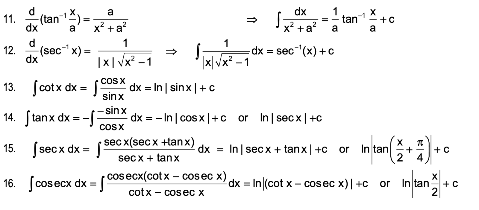
7. d/dx ( tan x ) = sec² x ⇒ ∫ sec² x dx = tan x + c

8. d/dx ( cosec x ) = - cot x cosec x ⇒ ∫ cosec x cot x dx = -cosec x + c

9. d/dx ( cot x ) = - cosec² x ⇒ ∫ cosec² x dx = -cot x + c

10. d/dx ( sin^-1 x/a ) = 1 / root a² - x² ⇒ ∫ 1 root a² - x² dx = sin^-1 ( x/a ) + c

Standard Formulae

METHODS OF INTEGRATION

If the integrand is not a derivative of a known function, then the corresponding integrals cannot be found directly. In order to find the integral of complex problems, generally three rules of integration are used.

(1) Integration by substitution or by change of the independent variable.

(2) Integration by parts.

(3) Integration by partial fractions.

INTEGRATION BY SUBSTITUTION

Direct Substitution

Indirect Substitution

If the integrand is of the form f(x)g(x), where g(x) is a function of the integral of f(x), then put integral of f(x) = t.

INTEGRATION BY PARTS

If u and v be two functions of x, then integral of product of these two functions is given by:

∫ u v dx = u ∫ v dx - ∫ [du/dx ∫ v dx ] dx

(Inverse, Logarithmic, Algebraic, Trigonometric, Exponent)

In the above stated order, the function on the left is always chosen as the first function. This rule is called as ILATE e.g. In the integration of ∫ x sin x dx, x is taken as the first function and sinx is taken as the second function.

Ex.: ∫ sec (tan^–1 x) dx can be rewritten as

(A) ∫ sec² θ dθ where θ = tan^–1 x

(B) ∫ sec³ θ dθ where θ = tan^–1 x

(C) ∫ cot² θ dθ where θ = cos^–1 x

(D) ∫ sec θ dθ where θ = sin^–1 x

Solution:(B).

I = ∫ sec (tan^–1 x) dx Let tan^–1x = θ ⇒ x = tan θ ⇒ dx = sec²θ dθ

∴ I = ∫ sec³ θ dθ = sec θ ∫ sec² θ dθ – ∫ tan θ (sec θ tan θ) dθ

= sec θ tan θ – ∫ (sec² θ – 1) sec θ dθ
= sec θ tan θ – ∫ sec θ tan θ dθ + ∫ sec θ dθ
= sec θ tan θ – I + ln|sec θ + tan θ|

⇒ I = ½ [sec θ tan θ] + ½ ln|sec θ + tan θ| + c

An important result: In the integral ∫ g(x)e^xdx, if g(x) can be expressed as
g(x) = f(x) + f′(x) then ∫ e^x[f(x) + f′(x)]dx = e^xf(x) + c

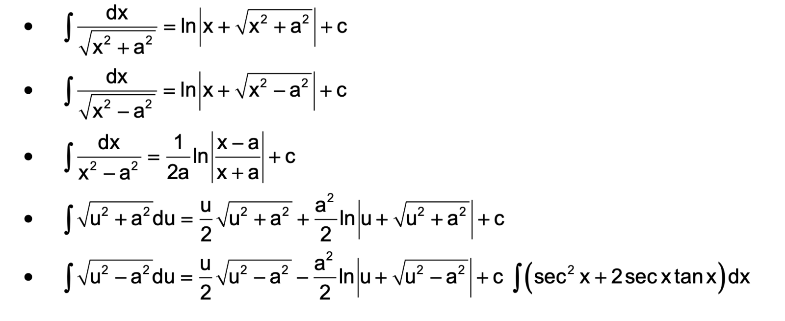
ALGEBRAIC INTEGRALS

Integrals of the form

∫ (px + q) / (ax² + bx + c) dx,  ∫ (px + q) / √(ax² + bx + c) dx,  ∫ (px + q) √(ax² + bx + c) dx

In these type of integrals we write px + q = ℓ (diff coefficient of ax² + bx + c) + m.

Find ℓ and m by comparing the coefficient of x and constant term on both sides of the identity. In this way the question will reduce to the sum of two integrals which can be integrated easily.

Integral of the type (ax² + bx + c) / (px² + qx + r)  or  (ax² + bx + c) / √(px² + qx + r)

In this case substitute ax² + bx + c = M (px² + qx + r) + N (2px + q) + R.

R. Find M, N, & R. The integration reduces to integration of three independent functions.

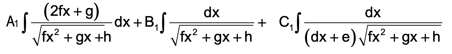
Integration of Irrational Algebraic Fractions

Here, we write, ax² + bx + c = A₁ (dx + e) ( 2fx + g) + B₁( dx + e) +C₁

where A₁, B₁ and C₁ are constants which can be obtained by comparing the coefficient of like terms on both sides. And given integral will reduce to the form

TRIGONOMETRIC INTEGRALS

Integrals of the form

(i)  ∫ (p cosx + q sinx + r) / (a cosx + b sinx + c) dx

(ii)  ∫ (p cosx + q sinx) / (a cosx + b sinx) dx

Rule for (i): In this integral express numerator as l (Denominator) + m (d.c. of denominator) + n. Find l, m, n by comparing the coefficients of sinx, cosx and constant term and split the integral into sum of three integrals.
l ∫ dx + m ∫ [d.c. of (Denominator)] / Denominator dx + n ∫ dx / (a cosx + b sinx + c)

Rule for (ii): Express numerator as l (denominator) + m (d.c. of denominator) and find l and m as above.

Integration of the Type: ∫(sin^Mx cos^Nx)dx
M & N ∈ natural numbers.

• If one of them is odd, then substitute for term of even power.
• If both are odd, substitute either of the term.
• If both are even, use trigonometric identities only.

Ex.: Evaluate ∫√sin x cos x dx

(A) ³⁄₂ (sin x)^3/5 + c
(B) ²⁄₃ (sin x)^3/2 + c
(C) ²⁄₃ (cos x)^3/2 + c
(D) ²⁄₃ (sin x)^1/4 + c

Solution: (B).

Put sin x = t
∫ t^1/2 dt = ²⁄₃ t^3/2 + c
= ²⁄₃ (sin x)^3/2 + c.

Formulas and Concepts 

1. For ∫ f(g(x)) g'(x) dx, put g(x) = t, provided ∫ f(t) dt exists.

2. ∫ u v dx = u ∫ v dx - ∫ [du/dx ∫ v dx] dx. For selecting ‘u’ use ILATE.

3. ∫ e^x [f(x) + f'(x)] dx = e^xf(x) + c.

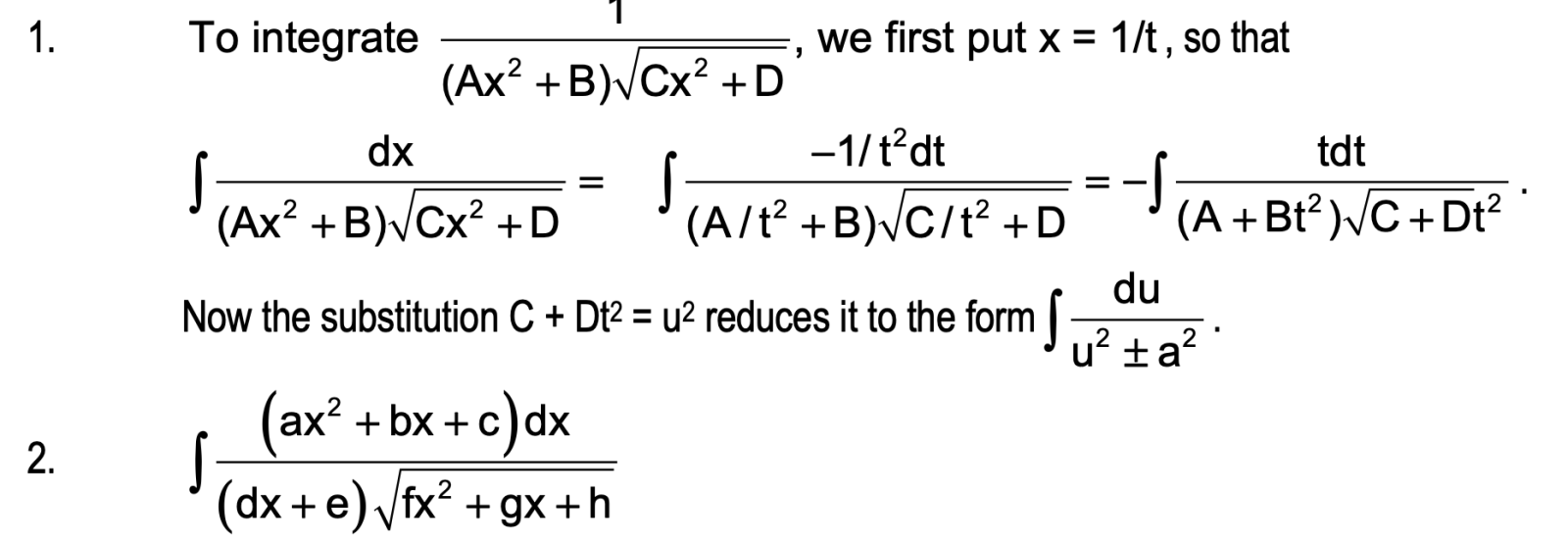
4. For 1/(A x² + B)√(C x² + D) , we first put x = 1/t, and then substitute C + D t² = u² to get the form ∫ du / (u² ± a²).

5. For ∫ (a x² + b x + c) dx / (dx + e)√(f x² + g x + h) . Put a x² + b x + c = A₁(dx + e)(2f x + g) + B₁(dx + e) + C₁ and proceed.

6. For ∫ p cos x + q sin x + r / a cos x + b sin x + c dx, express numerator as l (Denominator) + m (d.c. of denominator) + n.