The concept of limits forms the cornerstone of calculus, providing the mathematical framework for understanding continuous change and instantaneous rates. A limit describes the value that a function approaches as its input approaches a particular point, even if the function isn't defined at that exact point.
Formal Definition of Limits
In rigorous mathematical terms, for a function f(x), we say that the limit of f(x) as x approaches 'a' equals 'l' if, for every positive number ε (epsilon), however small, there exists a positive number δ (delta) such that whenever 0 < |x - a| < δ, we have |f(x) - l| < ε. This epsilon-delta definition ensures mathematical precision in limit calculations.
The notation lim (x → a) f(x) = l represents this fundamental concept. It's crucial to understand that x approaching a doesn't mean x equals a; rather, x assumes values increasingly close to 'a' without necessarily reaching it.
Left and Right Limits: Essential Conditions for Limit Existence
For a limit to exist at a point, both one-sided limits must exist and be equal. The left-hand limit, denoted as f(a-) or f(a - 0), represents the function's behavior as x approaches 'a' from values less than 'a'. Conversely, the right-hand limit, f(a+) or f(a + 0), describes the function's behavior as x approaches from values greater than 'a'.
Mathematically expressed:
- Left limit: f(a - 0) = lim(h→0) f(a - h), where h > 0
- Right limit: f(a + 0) = lim(h→0) f(a + h), where h > 0
The limit exists at x = a if and only if f(a - 0) = f(a + 0), and both are finite, or both approach the same infinity (either +∞ or -∞).
Key Formulas for Limits and Derivatives
| Formula Type | Mathematical Expression | Explanation |
|---|---|---|
| Trigonometric Limit | lim(x→0) sin x/x = 1 | Fundamental trigonometric limit (x in radians) |
| Exponential Limit (e) | lim(x→0) (1 + x)(1/x) = e | Definition of Euler's number |
| Alternative e Form | lim(x→∞) (1 + 1/x)x = e | Infinite approach to e |
| Natural Exponential | lim(x→0) (ex - 1)/x = 1 | Rate of change of exponential |
| Power Rule | lim(x→0) (ax - 1)/x = ln(a) | Logarithmic derivative relationship |
| Binomial Limit | lim(x→0) ((1+x)n - 1)/x = n | Power expansion principle |
| Logarithmic Limit | lim(x→0) ln(1+x)/x = 1 | Natural log approximation |
| Inverse Trig | lim(x→0) sin(-1)x/x = 1 | Arc-sine fundamental limit |
| Continuity Condition | lim(x→a-) f(x) = lim(x→a+) f(x) = f(a) | Function continuity requirement |
| Derivative Definition | f'(a) = lim(h→0) [f(a+h) - f(a)]/h | Fundamental derivative formula |
Six Essential Methods for Evaluating Limits
1. Factorization Method
When evaluating lim(x→a) φ(x)/ψ(x), factorize both numerator and denominator, cancel common factors containing 'a', then substitute x = a to find the limit. This method works particularly well for polynomial expressions.
2. Substitution Technique
Replace x with (a + h) in the expression, simplify both numerator and denominator, cancel common factors involving h, then evaluate the limit as h approaches zero. This technique proves valuable when direct substitution yields indeterminate forms.
3. L'Hospital's Rule Application
For indeterminate forms 0/0 or ∞/∞, L'Hospital's Rule states that lim(x→a) f(x)/g(x) = lim(x→a) f'(x)/g'(x), provided both functions are differentiable near point 'a' and the limit of the derivatives exists. This powerful tool simplifies complex limit evaluations significantly.
4. Rationalization Process
When dealing with irrational functions, multiplying by conjugate expressions helps eliminate radicals, making limit evaluation straightforward. This method is particularly effective for expressions involving square roots or higher-order radicals.
5. Infinite Limit Transformation
For limits as x approaches infinity, substitute x = 1/t, transforming the problem to evaluate as t approaches zero. This substitution often simplifies seemingly complex infinite limit problems.
6. Left and Right Limit Analysis
For piecewise functions or functions with different behaviors on either side of a point, evaluate both one-sided limits separately. The overall limit exists only when both sides agree.
Continuity and Differentiability: Building Blocks of Calculus
Understanding Continuity
A function exhibits continuity at point x = a when three conditions are satisfied simultaneously:
- The function f(a) is defined
- The limit lim(x→a) f(x) exists
- The limit equals the function value: lim(x→a) f(x) = f(a)
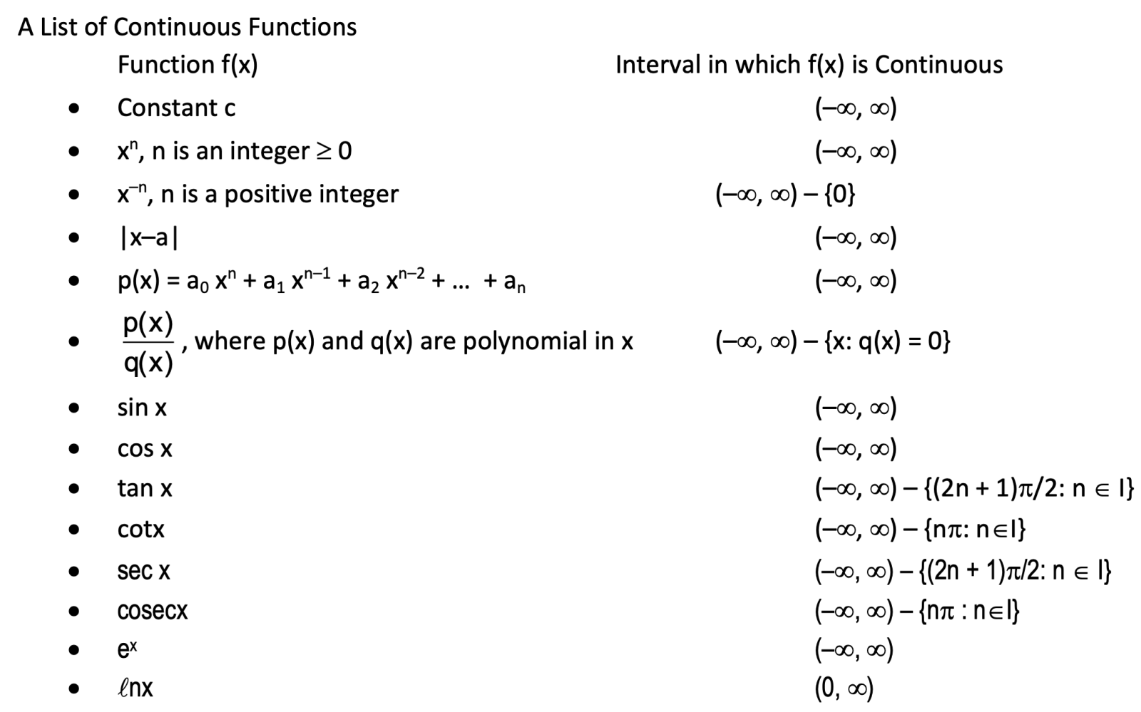
Common continuous functions include polynomials (continuous everywhere), trigonometric functions (continuous within their domains), exponential functions, and rational functions (except at points where denominators equal zero).
Also Check: NCERT Solutions Class 11 Math Chapter - 3 Trigonometric Functions
Differentiability Requirements
Differentiability represents a stronger condition than continuity. A function f(x) is differentiable at x = a when the limit of the difference quotient exists and is finite. The right-hand derivative Rf'(a) and left-hand derivative Lf'(a) must exist and be equal for differentiability to hold.
Key principle: Every differentiable function is continuous, but not every continuous function is differentiable. Sharp corners, cusps, or vertical tangents represent points where functions may be continuous but not differentiable.
Advanced Limit Evaluation Techniques
Handling Indeterminate Forms
Beyond the common 0/0 and ∞/∞ forms addressed by L'Hospital's Rule, other indeterminate forms include:
- 0 × ∞: Convert to 0/0 or ∞/∞ form through algebraic manipulation
- ∞ - ∞: Combine terms or rationalize to resolve
- 1^∞, 0^0, ∞^0: Use logarithmic transformation: f(x)^g(x) = e^(g(x)ln(f(x)))
The Sandwich Theorem Application
When direct methods fail, the Sandwich (Squeeze) Theorem provides an alternative approach. If g(x) ≤ f(x) ≤ h(x) near point 'a', and lim(x→a) g(x) = lim(x→a) h(x) = L, then lim(x→a) f(x) = L. This theorem proves particularly useful for oscillating functions and complex expressions.
Practical Applications and Problem-Solving Strategies
Understanding limits and derivatives enables solving real-world problems in physics (instantaneous velocity and acceleration), economics (marginal analysis), engineering (optimization), and biology (growth rates). The key to mastery lies in recognizing which evaluation method best suits each problem type and practicing diverse problem sets to build intuition.
For complex exponential limits of the form lim(x→a) [f(x)]^g(x), two specialized approaches apply:
- When lim(x→a) f(x) = 1, use the transformation e^(lim(x→a) g(x)[f(x)-1])
- When lim(x→a) f(x) ≠ 1, apply logarithmic properties: [f(x)]^g(x) = e^(g(x)·ln(f(x)))
These methods, combined with systematic practice and understanding of fundamental principles, provide the tools necessary for solving sophisticated calculus problems involving limits and derivatives.
DEFINITION OF LIMIT
Let f(x) be a function of x. If for every positive number ε, however small it may be, there exists a positive number δ, such that whenever 0 < |x - a| < δ, we have f(x) - l| <ε, then we say ‘f(x) tends to the limit l as x tends to a’, and we write:
Lim (x → a) f(x) I.
Meaning of (x → a)
Let x be a variable and ‘a’ be a constant. x assumes values nearer and nearer to ‘a’, then we say ‘x tends to a’ and write ‘x → a’ and it doesn’t mean x = a.
Condition for Existence of Limit: Left and Right Limit
Let y = f(x) be a given function, and x = a is the point under consideration. Left tendency of f(x) at x = a is called its left limit and right tendency is called its right limit.
Left tendency (left limit) is denoted by f(a − 0) or f(a–) and right tendency (right limit) is denoted by f(a + 0) or f(a+) and are written as:
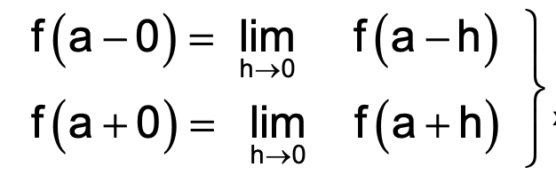
where ‘h’ is a small positive number.
Thus for the existence of the limit of f(x) at x = a, it is necessary and sufficient that f(a - 0) = f(a + 0), if these are finite or f(a - 0) and f(a + 0) both should be either + ∞ or − ∞.
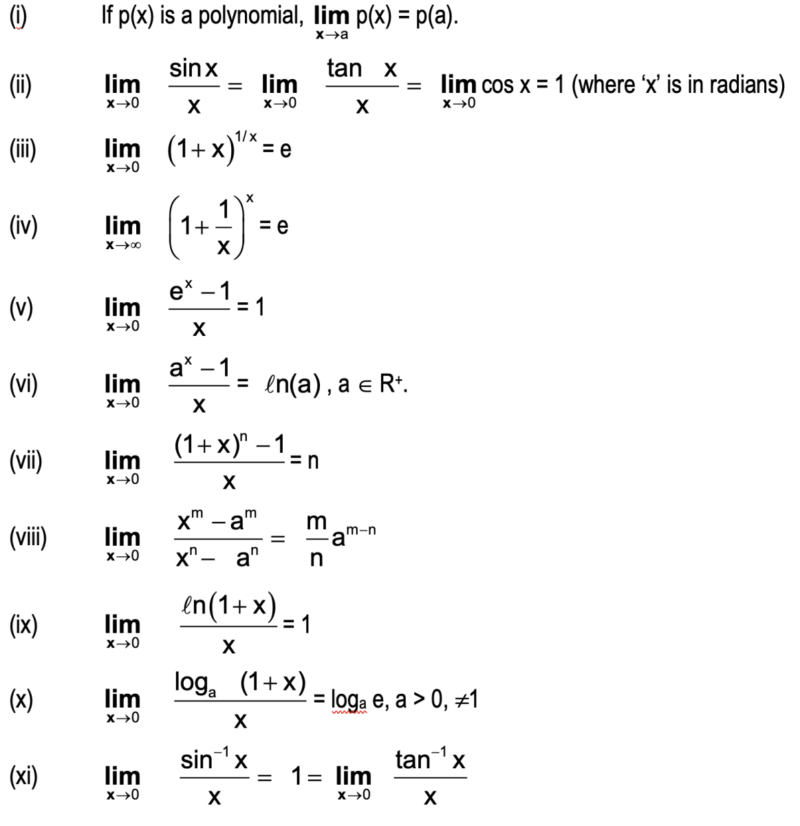
Frequently Used Limits
Evaluation of Limits (Working Rules)
- By factorization: To evaluate limx→aφ(x)/ψ(x), factorise both φ(x) and ψ(x), if possible, then cancel the common factor involving ‘a’ from the numerator and the denominator. In the last, obtain the limit by substituting ‘x’ for ‘a’.
- By Substitution: To evaluate limx→a f(x), put x = a + h and simplify the numerator and denominator, then cancel the common factor involving h in the numerator and denominator. In the last obtain the limit by substituting h = 0.
- By L–Hospital’s Rule: Apply L–Hospital’s rule to the form 0/0 or ∞/∞.
- By Rationalisation: In case if numerator or denominator (or both) are irrational functions, rationalisation of numerator or denominator (or both) helps to obtain the limits of the function.
- In case of limits x → ∞, put x = 1/t or t = 1/x, so that t → 0 when x → ∞ and proceed as usual.
- To find the limit by finding L.H.L and R.H.L.: We evaluate the limit of a function f(x) at x → a by finding its right hand limit (R.H.L) and left hand limit (L.H.L) in the special case when the values of f(x) are given by different functions of x for x < a and for x ≥ a.
Here we discuss two different cases,
(a) When limx→a f(x) = 1:
In this case,
limx→a [f(x)]g(x) = limx→a [1 + f(x) - 1]g(x)
= limx→a ( [1 + f(x) - 1]1/(f(x)-1) )g(x)(f(x)-1)
= elimx→a g(x)(f(x)-1)
because, limx→a ( [1 + f(x) - 1]1/(f(x)-1) ) = e
(b) When limx→a f(x) ≠ 1 but f(x) is positive in the neighbourhood of x = a.
In this case we write,
(f(x))g(x) = eg(x)·ln(f(x))
⇒ limx→a [f(x)]g(x) = elimx→a g(x)·ln(f(x))
Remark:
- If f(x) is not throughout positive in the neighbourhood of x = a, then limx→a (f(x))g(x) will not exist. Because in this case function will not be defined in the neighbourhood of x = a.
L'Hospital’s Rule
Let f(x) and g(x) be two functions differentiable in the neighbourhood of the point a, except at the point ‘a’ itself. If limx→a f(x) = limx→a g(x) = 0. Or, limx→a f(x) = limx→a g(x) = ∞. Then limx→a [f(x)/g(x)] = limx→a [f'(x)/g'(x)] provided that the limit on the right exist as a finite number or is ±∞.
- L’Hospitals rule is not always useful. Consider the example, limx → ∞ (x + sin x) / (x - sin x) (form ∞/∞).
Here, if we apply L’Hospital’s rule, then limx → ∞ (x + sin x) / (x - sin x) = limx → ∞ (1 + cos x) / (1 - cos x) .
Now, both the numerator and denominator are undefined because limx → ∞ cos x doesn’t exist.
We can find this limit as follows:
limx → ∞ (x + sin x) / (x - sin x) = limx → ∞ (1 + (sin x / x)) / (1 - (sin x / x)) = (1 + 0) / (1 - 0) = 1 since limx → ∞ (sin x / x) = 0 .
Use of Sandwich Theorem in Solving Problems
Sandwich theorem helps in calculating the limits, when limits can not be calculated using the usual methods. The following illustration would make the procedure clear,
CONTINUITY OF A FUNCTION
A function f(x) is said to be continuous at x = a if
limx→a- f(x) = limx→a+ f(x) = f(a)
If f(x) is not continuous at x = a, we say that f(x) is discontinuous at x = a.
f(x) will be discontinuous at x = a in any of the following cases:
(i) limx→a- f(x) and limx→a+ f(x) exist but are not equal.
(ii) limx→a- f(x) and limx→a+ f(x) exist and are equal but not equal to f(a).
(iii) f(a) is not defined.
(iv) At least one of the limits does not exist.
DIFFERENTIABILITY
Let y = f(x) be continuous in (a, b). Then the derivative or differential of f(x) at x ∈ (a, b), denoted by dy/dx or f′(x), and is defined as
provided the limit exists and is finite.
Right hand derivative
Right hand derivative of f(x) at x = a is denoted by, Rf′(a) or f′(a+) and defined as
Left hand derivative
Left hand derivative of f(x) at x = a is denoted by Lf′(a) or f′(a−) and is defined as
Clearly, f(x) is differentiable at x = a if and only if Rf′(a) = Lf′(a).
Note:
If a function f(x) is differentiable at x = a then it is also continuous at x = a. But if a function is continuous at a point, it is not necessarily differentiable at that point.
Formulas and Concepts
- For the existence of the limit at x = a, f(x) need not be defined at x = a. However if f(a) exists, limit need not exist or even if it exists then it need not be equal to f(a). limx→a f(g(x)) = f(limx→a g(x)) = f(ℓ2) , if and only if f(x) is continuous at x = ℓ2.
- Right hand derivative of f(x) at x = a is denoted by, Rf'(a) or f'(a+) and is defined as
R f'(a) = limh→0 [f(a+h) – f(a)] / h, h > 0.
- Left hand derivative of f(x) at x = a is denoted by Lf'(a) or f'(a–) and is defined as
L f'(a) = limh→0 [f(a–h) – f(a)] / –h, h > 0.
- f(x) is differentiable at x = a if and only if R f'(a) = L f'(a).
- L' Hospital's Rule
We have dealt with problems which had indeterminate form either 0/0 or ∞/∞.
The other indeterminate forms are ∞ − ∞, 0·∞, 00, ∞0, 1∞.
We state below a rule, called L' Hospital's Rule, meant for problems on limit of the form 0/0 or ∞/∞.
Let f(x) and g(x) be functions differentiable in the neighbourhood of the point a, except may be at the point a itself. If
limx→a f(x) = 0 = limx→a g(x)
or,
limx→a f(x) = ∞ = limx→a g(x),
then
limx→af(x)/g(x) = limx→af'(x)/g'(x)
provided that the limit on the right either exists as a finite number or is ±∞.
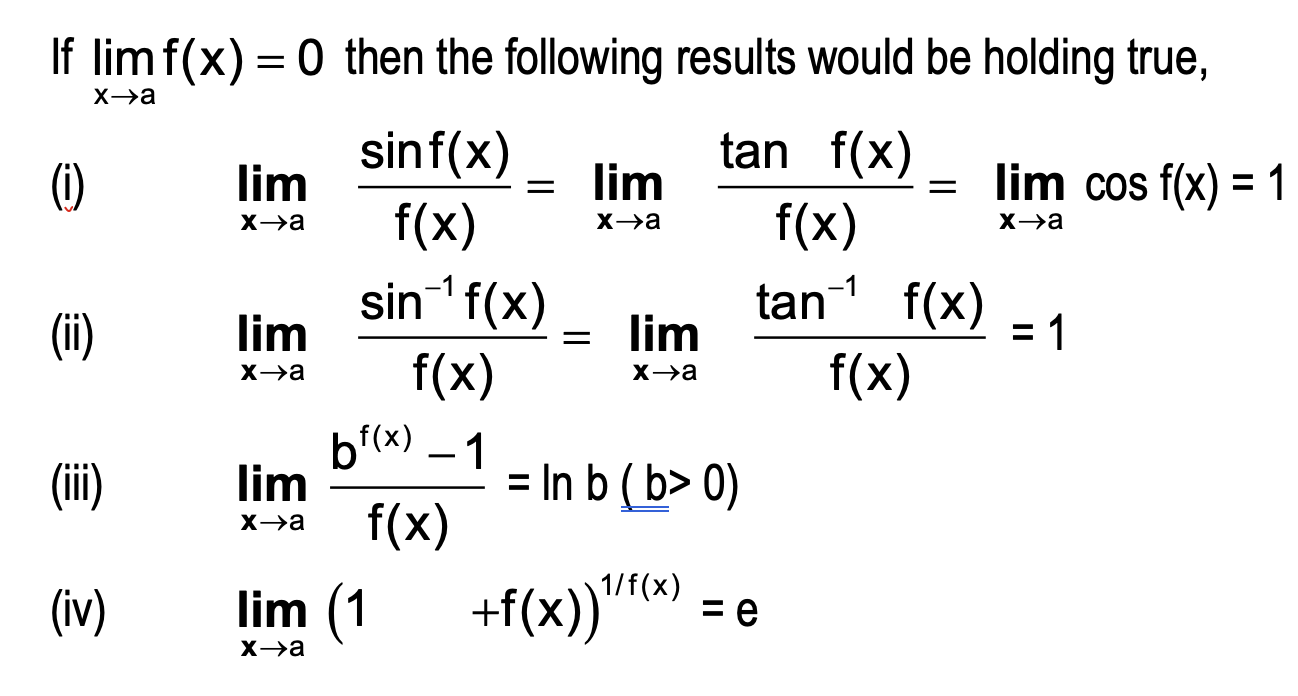
- If limx → a f(x) = 0, then the following results will be holding true:
- limx → a ¼sin f(x)⁄f(x)¾ = limx → a ¼tan f(x)⁄f(x)¾ = limx → a cos f(x) = 1
- limx → a ¼sin−1 f(x)⁄f(x)¾ = limx → a ¼tan−1 f(x)⁄f(x)¾ = 1
- limx → a ¼bf(x) - 1⁄f(x)¾ = ln b (b > 0)
- limx → a (1 + f(x))1/f(x) = e