The sample space (S) is the set of all possible outcomes of a random experiment. To find it, list every possible result that could occur. For example: Tossing a coin: S = {Head, Tail} Rolling a die: S = {1, 2, 3, 4, 5, 6} Drawing a card from a deck: S = {all 52 cards} Tossing two coins: S = {HH, HT, TH, TT} Each individual element in the sample space is called a sample point. Understanding the sample space is crucial for calculating probabilities accurately, as it represents the denominator in the basic probability formula.

The sample space (S) is the set of all possible outcomes of a random experiment. To find it, list every possible result that could occur. For example: Tossing a coin: S = {Head, Tail} Rolling a die: S = {1, 2, 3, 4, 5, 6} Drawing a card from a deck: S = {all 52 cards} Tossing two coins: S = {HH, HT, TH, TT} Each individual element in the sample space is called a sample point. Understanding the sample space is crucial for calculating probabilities accurately, as it represents the denominator in the basic probability formula.

Mutually exclusive events are events that cannot occur simultaneously. If event A happens, event B cannot happen at the same time. For example, when rolling a die, getting an even number and getting an odd number are mutually exclusive events.For mutually exclusive events A and B: P(A ∩ B) = 0 (intersection is empty) P(A ∪ B) = P(A) + P(B) (addition rule simplifies) This is different from the general addition rule: P(A ∪ B) = P(A) + P(B) - P(A ∩ B), where the intersection term becomes zero for mutually exclusive events.

Mutually exclusive events are events that cannot occur simultaneously. If event A happens, event B cannot happen at the same time. For example, when rolling a die, getting an even number and getting an odd number are mutually exclusive events.For mutually exclusive events A and B: P(A ∩ B) = 0 (intersection is empty) P(A ∪ B) = P(A) + P(B) (addition rule simplifies) This is different from the general addition rule: P(A ∪ B) = P(A) + P(B) - P(A ∩ B), where the intersection term becomes zero for mutually exclusive events.

Two events A and B are independent if the occurrence of one event does not affect the probability of the other event occurring. You can determine independence using these criteria: P(A|B) = P(A) - knowing B occurred doesn't change A's probability P(B|A) = P(B) - knowing A occurred doesn't change B's probability P(A ∩ B) = P(A) × P(B) - multiplication rule for independent events Example: When tossing two coins, the result of the first coin doesn't affect the second coin's outcome, making these independent events. However, drawing two cards from a deck without replacement creates dependent events, as the first draw affects the second draw's probability.

Two events A and B are independent if the occurrence of one event does not affect the probability of the other event occurring. You can determine independence using these criteria: P(A|B) = P(A) - knowing B occurred doesn't change A's probability P(B|A) = P(B) - knowing A occurred doesn't change B's probability P(A ∩ B) = P(A) × P(B) - multiplication rule for independent events Example: When tossing two coins, the result of the first coin doesn't affect the second coin's outcome, making these independent events. However, drawing two cards from a deck without replacement creates dependent events, as the first draw affects the second draw's probability.

Conditional probability is the probability of an event B occurring given that event A has already occurred, denoted as P(B|A). The formula is: P(B|A) = P(A ∩ B) / P(A) , where P(A) > 0You use conditional probability when: Information about one event affects another event's likelihood Events are dependent on each other You need to update probability based on new information Example: If you draw a card from a deck and it's red, what's the probability it's a heart? Here, P(Heart|Red) = P(Heart ∩ Red) / P(Red) = (13/52) / (26/52) = 1/2, since all hearts are red cards.

Conditional probability is the probability of an event B occurring given that event A has already occurred, denoted as P(B|A). The formula is: P(B|A) = P(A ∩ B) / P(A) , where P(A) > 0You use conditional probability when: Information about one event affects another event's likelihood Events are dependent on each other You need to update probability based on new information Example: If you draw a card from a deck and it's red, what's the probability it's a heart? Here, P(Heart|Red) = P(Heart ∩ Red) / P(Red) = (13/52) / (26/52) = 1/2, since all hearts are red cards.

Bayes' theorem helps find the probability of a cause given an observed effect. The formula is: P(Ai|A) = [P(Ai) × P(A|Ai)] / [∑ P(Aj) × P(A|Aj)] Steps to solve Bayes' theorem problems: Identify the causes (Ai) and the observed effect (A) Find prior probabilities P(Ai) for each cause Find conditional probabilities P(A|Ai) for each cause Apply the total probability theorem to find P(A) Calculate the posterior probability using Bayes' formula Example: If a diagnostic test has 90% accuracy and a disease affects 1% of the population, Bayes' theorem helps calculate the actual probability of having the disease given a positive test result.

Bayes' theorem helps find the probability of a cause given an observed effect. The formula is: P(Ai|A) = [P(Ai) × P(A|Ai)] / [∑ P(Aj) × P(A|Aj)] Steps to solve Bayes' theorem problems: Identify the causes (Ai) and the observed effect (A) Find prior probabilities P(Ai) for each cause Find conditional probabilities P(A|Ai) for each cause Apply the total probability theorem to find P(A) Calculate the posterior probability using Bayes' formula Example: If a diagnostic test has 90% accuracy and a disease affects 1% of the population, Bayes' theorem helps calculate the actual probability of having the disease given a positive test result.

Here are the essential probability formulas you must memorize for CBSE Class 11: Basic Formulas: Basic probability: P(A) = n/N Complement rule: P(A') = 1 - P(A) Addition rule: P(A ∪ B) = P(A) + P(B) - P(A ∩ B) Advanced Formulas: Conditional probability: P(B|A) = P(A ∩ B) / P(A) Multiplication rule: P(A ∩ B) = P(A) × P(B|A) Independent events: P(A ∩ B) = P(A) × P(B) Total probability: P(A) = ∑ P(Ai) × P(A|Ai) Bayes' theorem: P(Ai|A) = [P(Ai) × P(A|Ai)] / P(A) Practice applying these formulas with various problem types to build confidence and speed during exams.

Here are the essential probability formulas you must memorize for CBSE Class 11: Basic Formulas: Basic probability: P(A) = n/N Complement rule: P(A') = 1 - P(A) Addition rule: P(A ∪ B) = P(A) + P(B) - P(A ∩ B) Advanced Formulas: Conditional probability: P(B|A) = P(A ∩ B) / P(A) Multiplication rule: P(A ∩ B) = P(A) × P(B|A) Independent events: P(A ∩ B) = P(A) × P(B) Total probability: P(A) = ∑ P(Ai) × P(A|Ai) Bayes' theorem: P(Ai|A) = [P(Ai) × P(A|Ai)] / P(A) Practice applying these formulas with various problem types to build confidence and speed during exams.

When drawing cards without replacement , each draw affects subsequent draws, creating dependent events. Use conditional probability: For two cards drawn without replacement: P(both events) = P(first event) × P(second event|first event occurred) Example: Probability of drawing two aces from a standard deck: P(first ace) = 4/52 P(second ace|first was ace) = 3/51 (only 3 aces left in 51 cards) P(both aces) = (4/52) × (3/51) = 12/2652 = 1/221 Key difference: With replacement, probabilities remain constant. Without replacement, adjust the numerator and denominator for each subsequent draw based on what was previously drawn.

When drawing cards without replacement , each draw affects subsequent draws, creating dependent events. Use conditional probability: For two cards drawn without replacement: P(both events) = P(first event) × P(second event|first event occurred) Example: Probability of drawing two aces from a standard deck: P(first ace) = 4/52 P(second ace|first was ace) = 3/51 (only 3 aces left in 51 cards) P(both aces) = (4/52) × (3/51) = 12/2652 = 1/221 Key difference: With replacement, probabilities remain constant. Without replacement, adjust the numerator and denominator for each subsequent draw based on what was previously drawn.

Binomial distribution models experiments with repeated independent trials having exactly two outcomes (success/failure). A binomial experiment must satisfy these conditions: Fixed number of trials (n) Two possible outcomes per trial (success/failure) Constant probability of success (p) in each trial Independent trials - one trial doesn't affect others Binomial probability formula: P(X = r) = nCr × pr × qn-rWhere: n = number of trials r = number of successes desired p = probability of success per trial q = (1-p) = probability of failure per trial Examples: Tossing coins multiple times, multiple-choice test answers, manufacturing defects in production batches.

Binomial distribution models experiments with repeated independent trials having exactly two outcomes (success/failure). A binomial experiment must satisfy these conditions: Fixed number of trials (n) Two possible outcomes per trial (success/failure) Constant probability of success (p) in each trial Independent trials - one trial doesn't affect others Binomial probability formula: P(X = r) = nCr × pr × qn-rWhere: n = number of trials r = number of successes desired p = probability of success per trial q = (1-p) = probability of failure per trial Examples: Tossing coins multiple times, multiple-choice test answers, manufacturing defects in production batches.

Students frequently make these probability mistakes: Conceptual Errors: Confusing P(A|B) with P(B|A) - these are generally different values Assuming events are independent when they're actually dependent Mixing up mutually exclusive and independent events Calculation Errors: Using wrong formulas for specific problem types Forgetting to subtract P(A ∩ B) in the addition rule Incorrectly calculating combinations and permutations Setup Mistakes: Not clearly defining the sample space Misidentifying favorable outcomes Incorrectly applying conditional probability concepts Prevention Tips: Read problems carefully, draw diagrams when helpful, clearly define events, and always check if your probability values are between 0 and 1.

Students frequently make these probability mistakes: Conceptual Errors: Confusing P(A|B) with P(B|A) - these are generally different values Assuming events are independent when they're actually dependent Mixing up mutually exclusive and independent events Calculation Errors: Using wrong formulas for specific problem types Forgetting to subtract P(A ∩ B) in the addition rule Incorrectly calculating combinations and permutations Setup Mistakes: Not clearly defining the sample space Misidentifying favorable outcomes Incorrectly applying conditional probability concepts Prevention Tips: Read problems carefully, draw diagrams when helpful, clearly define events, and always check if your probability values are between 0 and 1.

Follow this systematic approach for probability exam preparation: Foundation Building: Master basic definitions (sample space, events, probability) Memorize key formulas and understand when to apply each Practice set theory operations and Venn diagrams Problem Practice: Start with simple problems and gradually increase complexity Practice different problem types: cards, dice, coins, real-world scenarios Focus on word problems requiring formula selection skills Time yourself to build speed and accuracy Advanced Preparation: Master conditional probability and Bayes' theorem thoroughly Practice binomial distribution problems Solve previous year CBSE questions and sample papers Create formula sheets for quick reference Exam Strategy: Read questions twice, identify the problem type, draw diagrams when helpful, show all steps clearly, and verify answers make logical sense.

Follow this systematic approach for probability exam preparation: Foundation Building: Master basic definitions (sample space, events, probability) Memorize key formulas and understand when to apply each Practice set theory operations and Venn diagrams Problem Practice: Start with simple problems and gradually increase complexity Practice different problem types: cards, dice, coins, real-world scenarios Focus on word problems requiring formula selection skills Time yourself to build speed and accuracy Advanced Preparation: Master conditional probability and Bayes' theorem thoroughly Practice binomial distribution problems Solve previous year CBSE questions and sample papers Create formula sheets for quick reference Exam Strategy: Read questions twice, identify the problem type, draw diagrams when helpful, show all steps clearly, and verify answers make logical sense.

For problems with multiple events, follow this systematic approach: Step 1: Identify Event Relationships Determine if events are mutually exclusive, independent, or dependent Check if events form partitions of the sample space Step 2: Choose Appropriate Formulas Union (A ∪ B): Use P(A ∪ B) = P(A) + P(B) - P(A ∩ B) Intersection (A ∩ B): Use multiplication rules based on independence Three events: Apply extended addition rule with all intersections Step 3: Calculate Step by Step Find individual event probabilities first Calculate intersections using conditional probability when needed Apply the chosen formula systematically Example: For P(A ∪ B ∪ C), you need seven terms: three individual probabilities, three pairwise intersections, and one triple intersection. Organize calculations clearly to avoid errors.

For problems with multiple events, follow this systematic approach: Step 1: Identify Event Relationships Determine if events are mutually exclusive, independent, or dependent Check if events form partitions of the sample space Step 2: Choose Appropriate Formulas Union (A ∪ B): Use P(A ∪ B) = P(A) + P(B) - P(A ∩ B) Intersection (A ∩ B): Use multiplication rules based on independence Three events: Apply extended addition rule with all intersections Step 3: Calculate Step by Step Find individual event probabilities first Calculate intersections using conditional probability when needed Apply the chosen formula systematically Example: For P(A ∪ B ∪ C), you need seven terms: three individual probabilities, three pairwise intersections, and one triple intersection. Organize calculations clearly to avoid errors.

Permutations and combinations are counting techniques essential for probability calculations: Permutations (nPr): Order matters Formula: nPr = n!/(n-r)! Used when arrangement sequence is important Example: Selecting and arranging 3 students from 10 for class positions Combinations (nCr): Order doesn't matter Formula: nCr = n!/(r!(n-r)!) Used when selection without regard to order Example: Choosing 3 students from 10 for a committee In Probability Context: Use permutations when calculating arrangements (like seating arrangements) Use combinations for selections (like drawing cards, choosing committee members) Remember: nCr ≤ nPr always, since removing order restrictions reduces possible outcomes Quick Check: Ask "Does the order of selection matter?" to choose between permutations and combinations.

Permutations and combinations are counting techniques essential for probability calculations: Permutations (nPr): Order matters Formula: nPr = n!/(n-r)! Used when arrangement sequence is important Example: Selecting and arranging 3 students from 10 for class positions Combinations (nCr): Order doesn't matter Formula: nCr = n!/(r!(n-r)!) Used when selection without regard to order Example: Choosing 3 students from 10 for a committee In Probability Context: Use permutations when calculating arrangements (like seating arrangements) Use combinations for selections (like drawing cards, choosing committee members) Remember: nCr ≤ nPr always, since removing order restrictions reduces possible outcomes Quick Check: Ask "Does the order of selection matter?" to choose between permutations and combinations.

The replacement condition significantly affects probability calculations: With Replacement: Sample space remains constant for each draw Events are independent Probabilities stay the same for each trial Use basic multiplication: P(A and B) = P(A) × P(B) Without Replacement: Sample space decreases with each draw Events become dependent Probabilities change based on previous outcomes Use conditional probability: P(A and B) = P(A) × P(B|A) Example Comparison: Drawing 2 red balls from 10 balls (6 red, 4 blue): With replacement: P(both red) = (6/10) × (6/10) = 36/100 Without replacement: P(both red) = (6/10) × (5/9) = 30/90 = 1/3Always check the problem statement carefully to determine whether items are replaced after each draw, as this fundamentally changes your calculation approach.

The replacement condition significantly affects probability calculations: With Replacement: Sample space remains constant for each draw Events are independent Probabilities stay the same for each trial Use basic multiplication: P(A and B) = P(A) × P(B) Without Replacement: Sample space decreases with each draw Events become dependent Probabilities change based on previous outcomes Use conditional probability: P(A and B) = P(A) × P(B|A) Example Comparison: Drawing 2 red balls from 10 balls (6 red, 4 blue): With replacement: P(both red) = (6/10) × (6/10) = 36/100 Without replacement: P(both red) = (6/10) × (5/9) = 30/90 = 1/3Always check the problem statement carefully to determine whether items are replaced after each draw, as this fundamentally changes your calculation approach.

Probability Theory: Complete Guide to Random Experiments, Events, and Statistical Analysis

Introduction to Probability and Random Experiments

Probability theory forms the mathematical foundation for understanding uncertainty and randomness in various fields, from statistics and data science to finance and engineering. At its core, probability quantifies the likelihood of events occurring in situations where outcomes cannot be predicted with certainty. A random experiment represents any process whose outcome cannot be determined beforehand, even though all possible outcomes are known. Classic examples include rolling dice, flipping coins, or drawing cards from a deck—each representing scenarios where chance governs the results.

The fundamental principle of probability states that if a random experiment can result in N equally likely outcomes, with exactly n outcomes favoring event A, then the probability of event A equals n/N. This ratio, bounded between 0 and 1, provides a mathematical framework for quantifying uncertainty. When probability equals 0, the event is impossible; when it equals 1, the event is certain to occur.

Sample Spaces, Events, and Their Classifications

The sample space (denoted as S) encompasses all possible outcomes of a random experiment, with each individual outcome called a sample point. Understanding sample spaces is crucial for probability calculations, as they define the universe of possibilities for any given experiment. For instance, when rolling two dice, the sample space contains 36 ordered pairs representing all possible combinations.

Events, which are subsets of the sample space, can be classified into several important categories. Simple events contain only one sample point, representing a single specific outcome. Compound events comprise multiple sample points and can be expressed as unions of simple events. Events may also be mutually exclusive (cannot occur simultaneously), independent (occurrence of one doesn't affect the other), or exhaustive (at least one must occur in any trial). These classifications are essential for applying the correct probability formulas and understanding the relationships between different outcomes.

Set Theory Principles in Probability

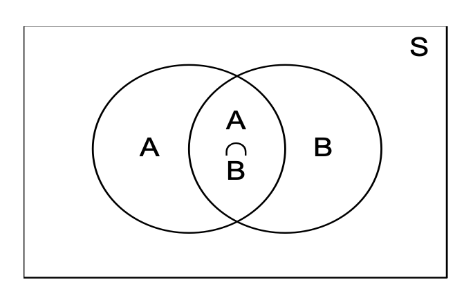
Probability theory extensively utilizes set operations to describe relationships between events. The union of events (A ∪ B) represents the occurrence of at least one event, while the intersection (A ∩ B) indicates simultaneous occurrence. The complement of an event (A' or Ā) represents its non-occurrence. These set-theoretic principles enable complex probability calculations through systematic application of fundamental rules.

The addition rule for probability states that P(A ∪ B) = P(A) + P(B) - P(A ∩ B), accounting for the overlap between events to avoid double-counting. For three events, this extends to include all pairwise intersections and the triple intersection. Understanding odds provides an alternative perspective: if m cases favor event A and n cases don't, the odds in favor equal m:n, while odds against equal n:m.

Conditional Probability and Independence

Conditional probability P(B|A) measures the likelihood of event B occurring given that event A has already occurred. This concept is fundamental in sequential processes and decision-making scenarios where prior information influences subsequent probabilities. Mathematically, P(B|A) = P(A ∩ B)/P(A), provided P(A) > 0. This formula reflects how the sample space effectively reduces to event A when calculating the conditional probability.

Independence between events represents a special case where P(B|A) = P(B), meaning knowledge of A's occurrence doesn't affect B's probability. For independent events, the multiplication rule simplifies to P(A ∩ B) = P(A) × P(B). This property is crucial in many applications, from quality control in manufacturing to risk assessment in insurance, where multiple independent factors contribute to overall outcomes.

Advanced Theorems: Total Probability and Bayes' Theorem

The Total Probability Theorem provides a systematic approach for calculating event probabilities when the sample space can be partitioned into mutually exclusive and exhaustive events. If A₁, A₂, ..., Aₙ partition the sample space, then P(A) = Σ P(Aᵢ) × P(A|Aᵢ). This theorem proves invaluable when direct probability calculation is difficult but conditional probabilities are known.

Bayes' Theorem, also known as the inverse probability theorem, enables updating probability assessments based on new evidence. Given that event A has occurred, the probability that it resulted from cause Aᵢ equals P(Aᵢ|A) = [P(Aᵢ) × P(A|Aᵢ)]/P(A). This theorem has profound applications in medical diagnosis, machine learning algorithms, spam filtering, and forensic analysis, where posterior probabilities must be calculated from prior knowledge and observed evidence.

Binomial Distribution and Repeated Trials

The binomial distribution models scenarios involving repeated independent trials with two possible outcomes (success or failure). When conducting n trials with success probability p and failure probability q = 1-p, the probability of exactly r successes follows the formula: P(X = r) = ⁿCᵣ × pʳ × qⁿ⁻ʳ. This distribution is fundamental in quality control, opinion polling, and biological experiments where binary outcomes are observed repeatedly.

The binomial coefficient ⁿCᵣ represents the number of ways to choose r successes from n trials, accounting for all possible orderings. Applications range from calculating defect rates in manufacturing to predicting election outcomes based on polling data. Understanding binomial probabilities enables researchers and analysts to make informed decisions about sample sizes and confidence levels in experimental design.

Practical Applications and Problem-Solving Strategies

Mastering probability requires systematic problem-solving approaches. First, clearly identify the sample space and relevant events. Second, determine whether events are independent, mutually exclusive, or conditional. Third, apply appropriate formulas based on these relationships. For complex problems, tree diagrams and probability tables can visualize relationships and organize calculations effectively.

Real-world applications demonstrate probability's versatility. In finance, probability models assess investment risks and option pricing. Healthcare professionals use conditional probability for diagnostic testing and treatment efficacy evaluation. Engineers apply reliability theory based on probability to design fail-safe systems. Data scientists leverage probability distributions for predictive modeling and statistical inference.

Quick Reference: Essential Probability Formulas

Formula Name	Mathematical Representation	Description
Basic Probability	P(A) = n/N	Ratio of favorable outcomes to total outcomes
Complement Rule	P(A') = 1 - P(A)	Probability of event not occurring
Addition Rule	P(A ∪ B) = P(A) + P(B) - P(A ∩ B)	Probability of at least one event occurring
Multiplication Rule (Independent)	P(A ∩ B) = P(A) × P(B)	Probability of both independent events occurring
Conditional Probability	P(B\|A) = P(A ∩ B)/P(A)	Probability of B given A has occurred
Total Probability	P(A) = Σ P(Aᵢ) × P(A\|Aᵢ)	Sum of weighted conditional probabilities
Bayes' Theorem	P(Aᵢ\|A) = [P(Aᵢ) × P(A\|Aᵢ)]/P(A)	Posterior probability given evidence
Binomial Probability	P(X = r) = ⁿCᵣ × pʳ × qⁿ⁻ʳ	Probability of r successes in n trials
Union of Complements	P(A' ∪ B') = 1 - P(A ∩ B)	Probability that at least one event doesn't occur
Three Events Union	P(A ∪ B ∪ C) = P(A) + P(B) + P(C) - P(A ∩ B) - P(A ∩ C) - P(B ∩ C) + P(A ∩ B ∩ C)	Inclusion-exclusion principle for three events

Random Experiment

An experiment, whose all possible outcomes are known in advance but the outcome of any specific performance can not predicted before the completion of the experiment, is known as random experiment.

Sample space and Sample Point

A set of all possible outcomes associated with same random experiment is called sample space and is usually denoted by ‘S’. Each element of a sample space is called a sample point.

Event

An event is a subset of sample space.

Simple Event and Compound Event

If an event is a set containing only one element of the sample space, then it is called a
simple event.

A compound event is one that can be represented as a union of simple events.

Probability

If a random experiment can result in any one of N different equally likely outcomes, and if exactly n of these outcomes favour A, then the probability of event A,

P(A) = n / N =
no. of favourable cases / total number of cases

0 ≤ P(A) ≤ 1, P(ϕ) = 0 and P(S) = 1.

Ex.: In a single cast with two fair dice the chance of throwing two 4’s is

(A) 1/18

(B) 1/9

(D) 1/12

Solution: (C).

There are 6 × 6 equally likely cases (as any face of any die may turn up) ⇒ 36 possible outcomes. For this event, only one outcome (4-4) is favourable.
∴ Probability = 1/36.

Mutually Exclusive Events

A set of events is said to be mutually exclusive if the occurrence of one of them precludes the occurrence of any of the other events.

Independent Events

Events are said to be independent if the occurrence or non-occurrence of one does not affect the occurrence or non-occurrence of other.

Exhaustive Event

A set of events is said to be exhaustive if the performance of random experiment always result in the occurrence of atleast one of them.

SET THEORETIC PRINCIPLES

If ‘A’ and ‘B’ be any two events of the sample space then

1. A ∪ B would stand for occurrence of at least one of them.
2. A ∩ B stands for simultaneous occurrence of A and B.
3. &overline;A (or A') stands for non-occurrence of A
4. &overline;A ∩ &overline;B (or A' ∩ B') stands for non-occurrence of both A and B.
5. If A and B are any two events, Then P(A ∪ B) = P(A) + P(B) - P(A ∩ B)
6. P(A') = 1 - P(A)
7. P(A' ∪ B') = 1 - P(A ∩ B)
8. If A, B, C are any three events of the sample space, then P(A ∪ B ∪ C) = P(A) + P(B) + P(C) – P(A ∩ B) – P(A ∩ C) – P(B ∩ C) + P(A ∩ B ∩ C)
9. If out of m + n equally likely, mutually exclusive and exhaustive cases, m cases are favourable to an event A and n are not favourable to the event A, m : n is called odds in favour of A, n : m is called odds against the event A.

Ex.: From a pack of 52 cards two cards are drawn at random. Then the probability that one card is of spade and one card is of diamond is

(A) ³/₁₇

(B) ²/₁₇

(D) none of these

Solution:(C).

Let E₂ be the event that one card is of spade and one is of diamond then n(E₂) = number of elements in E₂ = number of ways in which one card of spade can be selected out of 13 spade cards and one card of diamond can be selected out of 13 diamond cards. = ¹³C₁ × ¹³C₁ = 13 × 13 = 169

∴ P(E₂) = n(E₂)/n(S) = 169/1326 = 13/102

CONDITIONAL PROBABILITY

The probability of occurrence of an event B when it is known that some event A has occurred is called a conditional probability and is denoted by P(B/A). The symbol P(B/A) is usually read '‘the probability that B occurs given that A occurs” or ”simply probability of B, given A”.

conditional probability

Consider two events ‘A’ and ‘B’ of sample space S. When it is known that event ‘A’ has occurred, it means that sample space would reduce to the sample points representing event A. Now for P(B/A) we must look for the sample points representing the simultaneous occurrence of A and B i.e. sample points in A∩B.

⇒ P(B/A) = n(A ∩ B)n(A) = n(A ∩ B)n(S)n(A)n(S) = P(A ∩ B)P(A)

Thus P(B/A) = P(A ∩ B) P(A) , where 0 < P(A) ≤ 1; Similarly, P(A/B) = P(A ∩ B) P(B) , 0 < P(B) ≤ 1

Hence, P(A ∩ B) = { P(A) · P(B / A), P(A) > 0 P(B) · P(A / B), P(B) > 0 }

Independent Events

Two events A and B are said to be independent if occurrence or non-occurrence of one does not affect the occurrence or non-occurrence of the other,
i.e. P(B/A) = P(B), P(A) ≠ 0 similarly P(A/B) = P(A), P(B) ≠ 0
P(B/A) = P(A ∩ B) / P(A) = P(B) ⇒ P(A ∩ B) = P(A) · P(B)

Ex.: An event A₁ can happen with probability 0.4 and event A₂ can happen with probability 0.3, then the probability that exactly one of them happens is

(A) 0.24

(B) 0.7

(D) none of these

Solution: (C).

The probability that A₁ happens is p₁ = 0.4
∴ The probability that A₁ fails is 1 − p₁ = 0.6
Also the probability that A₂ happens is p₂ = 0.3
Now, the chance that A₁ happens and A₂ fails is p₁(1 − p₂) and the chance that A₁ fails and A₂ happens is p₂(1 − p₁)

The probability that one and only one of them happens is

p₁(1 - p₂) + p₂(1 - p₁) = p₁ + p₂ - 2p₁p₂ = 0.46

Total Probability Theorem and Bayes' Theorem

Partition of Sample Space

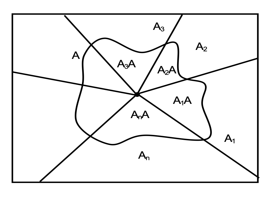
Consider a sample space ‘S’. Let A₁, A₂, ⋯, A_n be the set of mutually exclusive and exhaustive subsets of sample space S.
These A₁, A₂, ⋯, A_n events are said to partition the sample space into n parts.

We have A_i ∩ A_j = ∅ for i ≠ j, 1 ≤ i, j ≤ n

And ∑ⁿ_i=1 P(A_i) = 1

Probability

Total Probability Theorem

Let ‘A’ be any event of S. We can write A = (A₁ ∩ A) ∪ (A₂ ∩ A) ∪ … ∪ (A_n ∩ A). As A₁, A₂, …, A_n are mutually exclusive, (A₁ ∩ A), (A₂ ∩ A), …, (A_n ∩ A) would also be mutually exclusive.

⇒ P(A) = P(A₁ ∩ A) + P(A₂ ∩ A) + … + P(A_n ∩ A)

= P(A₁) · P(A / A₁) + P(A₂) · P(A / A₂) + … + P(A_n) · P(A / A_n)

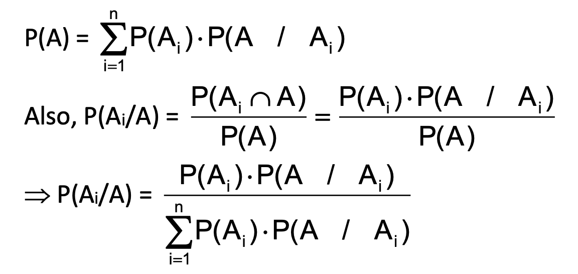
⇒ P(A) = ∑_i=1ⁿ P(A_i) · P(A / A_i)

This is known as the total probability of the event A.

Bayes’ Theorem

This theorem at times is also called inverse probability theorem.
Let us consider any event ‘A’ of sample space ‘S’ (as in the previous section). This event would have occurred due to the different causes (or due to the occurrence of any of the event A₁, A₂, ⋯ Aₙ).
Now, let us say that event A is found to have occurred and we have to find the probability that it has occurred to the occurrence of cause, say A_i.
That means we are interested in P(A_i/A). These types of problems are solved with the help of Bayes’ theorem.

From total probability theorem we get P(A) = ∑ⁿ_i=1 P(A_i) · P(A | A_i)

Also, P(A_i/A) = [P(A_i ∩ A)] / P(A) = [P(A_i) · P(A | A_i)] / P(A)

⇒ P(A_i/A) = [P(A_i) · P(A | A_i)] / [∑ⁿ_i=1 P(A_i) · P(A | A_i)]

This result is known as Bayes’ theorem.

BINOMIAL TRIALS AND BINOMIAL DISTRIBUTION

A probability distribution representing the binomial trials is said to be binomial distribution.

Let us consider a Binomial experiment which has been repeated ‘n’ times. Let the probability of success and failure in any trial be p and q respectively and we are interested in the probability of occurrence of exactly ‘r’ successes in these n trials. Now number of ways of choosing ‘r’ success in ‘n’ trials = ⁿC_r. Probability of ‘r’ successes and (n-r) failures is p^r×qⁿ^-^r. Thus probability of having exactly r successes = ⁿC_r×p^r×qⁿ^-^r.

Formulas and Concepts

If a random experiment can result in any one of N different equally likely outcomes, and if exactly n of these outcomes correspond to A, then the probability of event A,
P(A) = n / N.
If ‘A’ and ‘B’ be any two events of the sample space then
- A ∪ B would stand for occurrence of at least one of them.
- A (or A′ ∩ B′) stands for non-occurrence of both A and B.
- A ⊆ B stands for ‘the occurrence of A implies the occurrence of B’.
- A̅ (or A′) stands for non-occurrence of A.
- A̅ ∩ B̅ – P(A ∩ B)
- P(A′ ∪ B′) = 1 – P(A ∩ B)
- If out of m + n equally likely, mutually exclusive and exhaustive cases, m cases are favourable to an event and n are not favourable to the event A,
  m : n is called odds in favour of A, n : m is called odds against the event A.
The probability of occurrence of an event B when it is known that some event A has occurred is called a condition probability and is denoted by P(B/A).
P(B/A) = P(A ∩ B) / P(A), 0 < P(A) ≤ 1,P(A ∩ B) =

P(A) · P(B/A), P(A) > 0

P(B) · P(A/B), P(B) > 0

Let us consider a Binomial experiment which has been repeated ‘n’ times. Let the probability of success and failure in any trial be p and q respectively and we are interested in the probability of occurrence of exactly ‘r’ successes in these n trials. Now number of ways of choosing ‘r’ success in ‘n’ trials = nCr. Probability of ‘r’ successes and (n–r) failures is pr·qn–r. Thus probability of having exactly r successes = nCr·pr·qn–r
Let us consider any event ‘A’ of sample space ‘S’ (as in the previous section). Let us say that event A is found to have occurred and we have to find the probability that it has occurred to the occurrence of cause, say Ai.

Probability theory provides the mathematical framework for quantifying uncertainty and making informed decisions under randomness. From basic concepts of sample spaces and events to advanced applications of Bayes' theorem and binomial distributions, these principles underpin modern statistics, data science, and risk analysis. Mastery of probability enables professionals across disciplines to model complex systems, assess risks, and extract meaningful insights from data. Whether analyzing experimental results, developing machine learning algorithms, or making strategic business decisions, probability theory remains an indispensable tool for understanding and navigating uncertainty in our increasingly data-driven world.

Solved Problems

A number of six digits is written down at random. Probability that sum of digits of the number is even is

(A)1/2

(B) 3/8

(D) none of these

Sol. (A).

As we are considering all possible six digit numbers, half of these would have sum of their digits to be even and half of these would have sum of their digits to be odd. Hence the required probability would be 1/2.

Two small squares on a chess board are chosen at random. Probability that they have a common side is,

(A) 1/3

(B) 1/9

(D) none of these

Sol. (C)

There are 64 small squares on a chessboard.
⇒ Total number of ways to choose two squares = 64C₂ = 32.63
For favourable ways we must choose two consecutive small squares for any row or any column. ⇒ Number of favourable ways = (7×8)×2
favourable ways = (7×8)×2 ⇒ Required probability = ^7×8×2 ⁄ _32.63 = ¹ ⁄ ₁₈

3. Fifteen coupons are numbered 1, 2, 3, … 15. Seven coupons are selected at random one at a time with replacement. The probability that the largest number appearing on the selected coupon is 9, is

(A) (⁹⁄₁₆)⁶
(B) (⁸⁄₁₅)⁷
(C) (³⁄₅)⁷
(D) none of these

Sol. (D) Total ways = 15⁷

For favorable ways, we must have 7 coupons numbered from 1 to 9 so that '9' is selected at least once. Thus total number of favorable ways are, 9⁷ – 8⁷
⇒ Required probability = ^{9⁷ – 8⁷}⁄_15⁷

4. A fair coin is tossed a fixed number of times. If the probability of getting 7 heads is equal to getting 9 heads, then the probability of getting 2 heads is,

(A) 15/2⁸

(B) 2/15

(D) none of these

Sol. (C). Let coin be tossed 'n' times and X be the random variable representing the number of heads appearing in 'n' trials.
P(X = 7) = P(X = 9); ⇒ nC₇(1/2)^n-7 = nC₉(1/2)^n-9 × (1/2)⁹
⇒ nC₇ = nC₉ ⇒ n = 16; Now P(X = 2) = ¹⁶C₂(1/2)²(1/2)¹⁴
= ¹⁶C₂/2¹⁶ = (16×15)/2¹⁷ = 15/2¹³.

5. If the papers of 4 students can be checked by any one of the 7 teachers, then the probability that all the 4 papers are checked by exactly 2 teachers is

(A) 2/7

(B) 32/343

(D) none of these

Sol. (D) Total number of ways in which 4 papers can be distributed among 7 teachers = 7⁴
Now exactly 2 teachers out of 7 can be chosen in 7C₂ ways. And total number of ways in which 4 papers can be given to these 2 teachers (each one getting at least one) = (2⁴–2) =14

⇒ Total number of ways in which exactly 2 teachers check all four papers = 7C₂ × 14 = 21 × 14

⇒ Required probability = 21 ⋅ 14 7 4 = 3 ⋅ 2 7 2 = 6 49 .

6. A bag contains 5 white and 3 black balls. 4 balls are successively drawn out and not replaced. The probability that they are alternately of different colours is

(A) 1/196

(B) 2/7

(D) 13/56

Sol. (C). Required probability
= P(WBWB) + P(BWBW)
= ⁵/₈x ³/₇x⁴/₆x ²/₅+ ³/₈x ⁵/₇x ²/₆x ⁴/₅
= ¹/₇.

7. From a set of 100 cards numbered 1 to 100, one card is drawn at random. The probability that the number obtained on the card is divisible by 6 or 8 but not by 24 is

(A)⁶/₂₅

(B)¹/₄

(D) ¹/₅

Sol. (D). Let A: ‘’number is divisible by 6’’ and B: ‘’number is divisible by 8’’ then A ◠ B: ‘’number is divisible by 24’’.
⸫Required probability
= P(A OR B) – P(A ◠ B)
= P(A) + P(B) – P(A◠B) – P(A◠B)
=¹⁶/₁₀₀+¹²/₁₀₀-2(⁴/₁₀₀)=²⁰/₁₀₀=¹/₅.
(Note that a number is divisible both by 6 and 8 iff it is divisible by L.C.M. of 6 and 8 i.e. 24. From 1 to 100, there are 16 multiples of 6, 12 multiples of 8 and 4 multiples of 24)

8. Statistics show that a specific disease is fatal in 10% cases. Find the probability that out of six patients in a hospital, only 3 will die is

(A) 1458 x 10^-5

(B) 1458 x 10^-6

(D) 8748 x 10^-5

Sol. ( )It is a case of bernoullian trials where n = 6 and success may be defined as‘’ disease is fatal’’ so that
p=¹⁰/₁₀₀=¹/₁₀ and q = 1 -¹/₁₀=⁹/₁₀.
Required probability = P (3 successes)
=⁶C₃p²q³ =20(¹/₁₀)³(⁹/₁₀)³=¹⁴⁵⁸⁰/₁₀₆ .

Frequently Asked Questions

Probability is a measure of the likelihood that an event will occur, expressed as a number between 0 and 1. In CBSE Class 11, probability is calculated using the formula P(A) = n/N, where 'n' is the number of favorable outcomes and 'N' is the total number of equally likely outcomes.

For example, when rolling a fair die, the probability of getting a 4 is 1/6 because there's one favorable outcome (rolling 4) out of six total possible outcomes. The probability of an impossible event is 0, while the probability of a certain event is 1.

A random experiment is one where all possible outcomes are known in advance, but the specific outcome cannot be predicted before completing the experiment. Examples include tossing a coin, rolling dice, or drawing cards from a deck. In contrast, a deterministic experiment produces predictable results under identical conditions. For instance, dropping a ball from a specific height will always fall to the ground due to gravity. Random experiments form the foundation of probability theory and are essential for understanding uncertainty in mathematical contexts.

The sample space (S) is the set of all possible outcomes of a random experiment. To find it, list every possible result that could occur. For example:

Tossing a coin: S = {Head, Tail}
Rolling a die: S = {1, 2, 3, 4, 5, 6}
Drawing a card from a deck: S = {all 52 cards}
Tossing two coins: S = {HH, HT, TH, TT}

Each individual element in the sample space is called a sample point. Understanding the sample space is crucial for calculating probabilities accurately, as it represents the denominator in the basic probability formula.

S.no	Formulas List
1.	Sets Solutions
2.	Relations and Functions Solutions
3.	Trigonometric Functions Solutions
4.	Complex Numbers and Quadratic Equations Solutions
5.	Permutations and Combinations Solutions
6.	Binomial Theorem Solutions
7.	Sequences and Series Solutions
8.	Straight Lines Solutions
9.	Introduction to Three Dimensional Geometry Solutions
10.	Limits and Derivatives Solutions with Formulas and Methods

Probability Solutions - From Basic Concepts to Advanced Applications

Introduction to Probability and Random Experiments