Kinematics

Master CBSE Physics Kinematics with Expert-Crafted Notes That Make Complex Concepts Crystal Clear

Stop struggling with velocity, acceleration, and projectile motion. Our comprehensive CBSE notes break down every kinematics concept with step-by-step solutions, illustrated examples, and practice problems that guarantee better grades.

Frustrated with Confusing Physics Textbooks and Incomplete Class Notes?

Important Massage:

• Kinematics formulas seem impossible to remember and apply correctly
• Textbook explanations are too theoretical without practical problem-solving steps
• Class notes miss crucial details needed for board exams and competitive tests
• Practice problems lack detailed solutions that show the thinking process

Complete CBSE Kinematics Notes That Actually Make Sense

Important Messages:

• Clear Concept Building: From basic rest and motion to complex projectile trajectories
• Step-by-Step Problem Solving: Detailed solutions showing every calculation step
• Visual Learning: Graphs, diagrams, and illustrations for better understanding
• Exam-Ready Format: Aligned with CBSE syllabus and marking schemes

Trusted by Thousands of CBSE Students and Created by Home Tuition Experts

• Developed by experienced physics educators with proven track records
• Used successfully by students achieving 90+ marks in CBSE physics
• Comprehensive coverage from basic concepts to advanced applications
• Includes solved examples from actual CBSE and competitive exam questions

Everything You Need to Excel in CBSE Physics Kinematics

• Complete Topic Coverage: Motion in 1D, 2D, projectile motion, circular motion
• Formula Sheets: Quick reference guides for all kinematic equations
• Worked Examples: Over 50 solved problems with detailed explanations
• Practice Exercises: Additional problems with answers for self-assessment
• Graphical Analysis: Velocity-time, displacement-time graph interpretations
• Assignment Questions: Chapter-end problems matching CBSE exam patterns

REST & MOTION

Motion means change of position with time. When a body is at rest, its position does not change with time. But how do we describe the position of a body? In order to do that we need to describe it relative to another body for reference.

Thus, rest and motion are relative. A man sitting in a car moving at 55 kmph on highway is at rest relative to a co-passenger, while he is in motion relative to a person standing on the highway. 

In order to describe rest and motion, we select a frame of reference and then describe rest or motion relative to this frame of reference.

Motion can be of two types - transnational & rotational.

When a body moves such that it always remains parallel to itself throughout the motion it undergoes translation. When a body moves so that each point in the body maintains a constant distance relative to a fixed axis in space, the motion is rotation.

FRAMES OF REFERENCE

Two of the commonest kinds of coordinate system in use are

(a) Rectangular Cartesian Coordinates

(b) Polar coordinates

(I) 2 Dimensions

Cartesian:

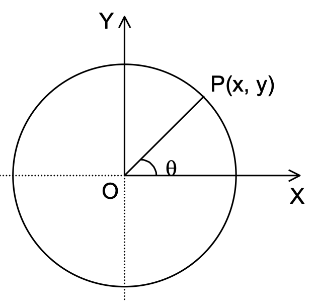
A point P with coordinates (x, y) in a rectangular cartesian coordinate system in figure is described by its position vector OP  also represented by vector r.

r = xî + yĵ, Where î, ĵ are unit vectors along x, y respectively.

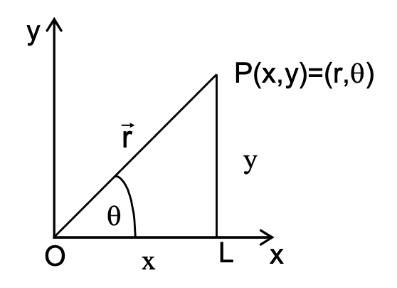
Here, x = r cos θ  y = r sin θ

vector r = r (cos θ vector i + sin θ vector j)

Polar:

If the initial ray is chosen to be OX, the point P can be described by the coordinates (r, θ) in the polar coordinate system.

r = rr̂
x = r cos θ
y = r sin θ

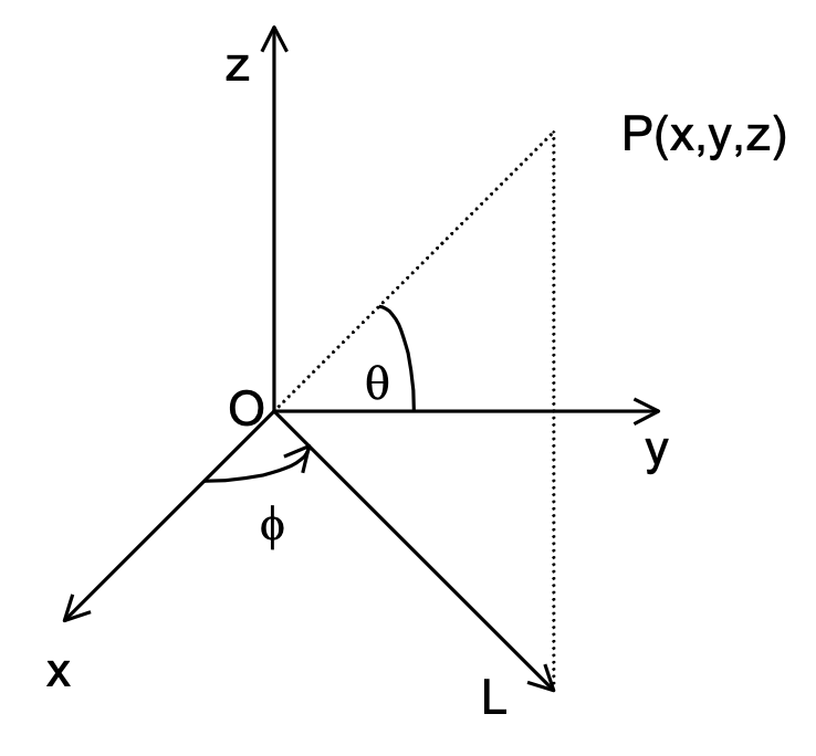
(II) 3 Dimensions

The simplest system of coordinate used in 3 dimensions is the rectangular cartesian coordinate system which consists of an origin O and three mutually perpendicular axes X, Y & Z.

A point P having coordinates (x, y, z) has the position vector:
r = vector OP = xî + yĵ + zk̂

DISPLACEMENT, VELOCITY & ACCELERATION

A particle P is said to be in motion with respect to a frame of reference K, if its position vector w.r.t. K changes with time.

r(t) = x(t)î + y(t)ĵ + z(t)k̂

Displacement

Particle Motion in Reference Frame

A particle P is said to be in motion with respect to a frame of reference K, if its position vector w.r.t. K changes with time.

Thus r ≡ r(t) ≡ x(t)i + y(t)j + z(t)k

Where x(t), y(t) & z(t) represent functions of time.

If a particle P moves from a point P₁ to a point P₂ in time t, its then displacement

of the particle P₁P₂ = OP₂ - OP₁

If P₁ ≡ P₁(x₁, y₁,z₁) and P₂ (x₂, y₂, z₂) then :

P₁P₂ = (x₂ - x₁)i + (y₂ - y₁)j + (z₂ - z₁)k

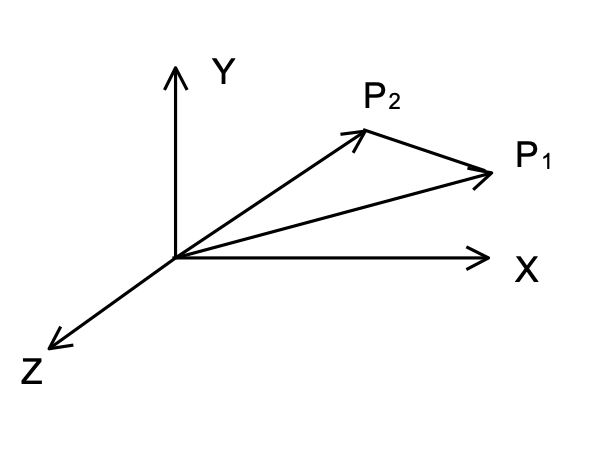
In 2-dimensions (or 1-dimension) the components would involve x, y coordinates (or x-coordinate) only.

The displacement of the particle vectors P₁P₂ does not depend on the path taken by the particle in moving from P₁ to P₂. It depends only on the initial and final position of the particle. It can be zero. Positive or negative.

Velocity of a particle is defined as the rate of change of the position vector (or displacement w.r.t a fixed origin O )

v = dr/dt = d/dt [x(t) î + y(t) ĵ + z(t) k̂]

= dx/dtî + dy/dtĵ + dz/dtk̂ ≡ v_xî + v_yĵ + v_zk̂

Of course, this defines the instantaneous velocity. It is a vector quantity.

The acceleration of a particle is the rate of change of velocity

a = dv/dt = d/dt (v_xî + v_yĵ + v_zk̂)

= dv_x/dtî + dv_y/dtĵ + dv_z/dtk̂

If a particle has a position vector r₁ and velocity v₁ at time t₁ and position vector r₂ & velocity v₂ at time t₂ then displacement between time t₁ and t₂ = r₂ − r₁

 

Average velocity = r₂ − r₁ /t₂ − t₁

Average acceleration = v₂ − v₁ /t₂ − t₁

Note that v₂ and v₁ are the instantaneous velocities at time t₂ and t₁.

It is also possible to represent the average velocity & average acceleration in terms of the instantaneous quantities and vice-versa (using limits).

Motion in 1 Dimension 

When a particle moves in a single dimension its motion can be described by means of a single coordinate. If the motion is linear, then we can use a linear coordinate, x, to describe its position at any time, t (figure)

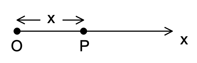
In general, x = x(t), a function of t the velocity, v(t) = dx/dt and acceleration,

a(t) = dv/dt = d²x/dt²

These are the fundamental kinematics equations of motion.

x = x(t), v = dx/dt

a = dv/dt = d²x/dt²

In order to illustrate the use of these equations, let us apply these to some examples:

(a) Uniformly accelerated motion → Freely falling body, Linear motion with uniform acceleration.

(b) Non-uniformly accelerated motion → SHM, Motion against a resisting force.

Motion of a body with uniform acceleration: In uniformly accelerated motion of an objected different relations are used to relate initial velocity final velocity (V) time (t), acceleration a and displacement s (distances). The commonly used equations are

V = u + at or v = u + at

V² = u² + 2as or V.V = u.u + 2a.s

S = ut + ¹⁄₂at² or S = ut + ¹⁄₂at²

The displacement of a body in the n^th second of its motion is

d_n = x_n - x_n-1 (x_n = displacement in n sec, x_n-1 = displacement in (n-1)sec.

= (un + ¹⁄₂ an²) - {u(n - 1) + ¹⁄₂a(n - 1)²}

d_n = u + ¹⁄₂ a(2n - 1)

Graphical Representation:

The displacement – time and velocity – time graphs of a motion give us a graphical representation of a motion of a particle. The shape of these graphs tells us about the kind of motion a particle has (see fig)

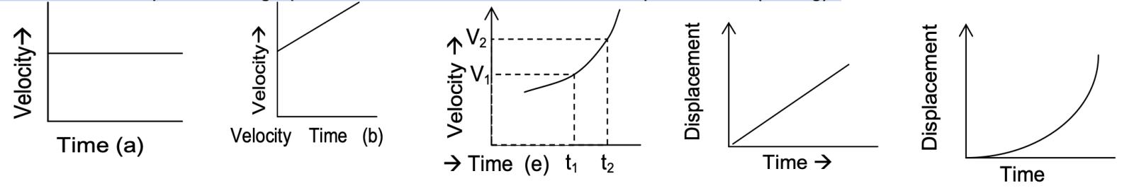
Fig : Curve (a) and (c) represent motion with a constant speed u. curves (b) and (d) represent motion with a uniform acceleration a starting with an initial speed u. curve (a) represent motion with a non uniform acceleration.

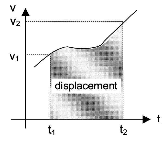
Velocity - time graph and equations of motion:

The velocity time graph gives three types of information.

i) The instantaneous velocity

ii) The slope of the tangent to the curve at any point gives instantaneous acceleration.

|a| = dv/dt = tan θ

iii) The area under the curve gives total displacement of the object.

s = ∫_t₁^t₂ v dt

 

The displacement time graph gives two type at information

1. The slope at the tangent to the curve at any point gives instantaneous velocity
2. The ratio of area under the curve and time interval gives average velocity.

Freely falling body under gravity

Consider a body P projected vertically upwards from the surface of the earth with an initial velocity, u (see figure)

The body rises to a maximum height at B and then returns (motion BC).

Even through we have shown the motion of the body as ABC, the actual path is always along the same time AB. The picture has been slightly modified for clarity.

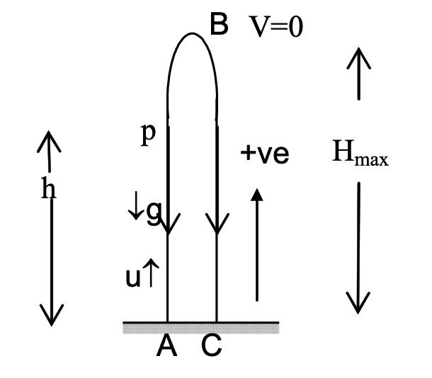
Let the displacement of the body (at P) at time t measured from its initial position A, be denoted by h.

Here

a = - g, S = + h, initial velocity = +u (upward direction = +Ve, downward direction –Ve
and starting point of body always takes as origin).

After time t,

v = u - gt. . . . (1)

h = ut + ¹/₂ (-g)t2 = ut - ¹/₂ gt2. . . . (2)

v2 = u2 + 2 (-g)h = u2 - 2gh. . . (3)

If tAB is the time taken by particle to travel from A to B then

tAB = u / g

and AB = ^u2/_2g = Hmax m (maximum height attained by particle)

When the body reaches the ground again (at the pt C), then displacement h = 0

0 = (u - ¹/₂ g tAC)tAC

tAC = ^2u/_g = 2 × tAB

It is called time at flight, t

Note :

In both the examples considered above, the acceleration is constant (or uniform). This may not always be true.

Motion in 2 Dimensions 

Motion of a projectile under the earth's gravity.

Consider a projectile projected with an initial velocity u at an angle q with the horizontal (see figure). The coordinate system is set as shown in order to analyse the motion of the projectile. The acceleration due to gravity, g, is uniform and the surface of the earth is considered to be flat.

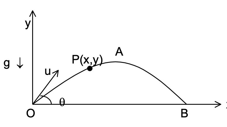
Let P(x, y) represent the position of the projectile after a time t from the time of projection.

Horizontal component of velocity u_x = ucosθ

Vertical component of velocity u_y = u sinθ

Acceleration due to gravity acting downwards vertically. Hence vertical component of velocity changes due to acceleration due to gravity. While horizontal component of velocity remains constant (ucosθ) during the complete motion.i.e. velocity of particle along x-axies is uniform motion and along y-axis is non uniform motion.

To calculate time of flight, we can find the time when vertical displacement is zero i.e.

0 = usinθt - 1/2gt²

⇒ t = 0 or t = 2usinθ/g

Thus time of flight T = 2usinθ/g

During this time horizontal component of velocity has taken the particle distance x

Where, x = ucosθ×T = u cosθ × 2usinθ/g = u² sin2θ/g

This distance, we call as range on horizontal plane

R = u² sin2θg

R_max = u²/g for θ = 45°

For given velocity same range can be obtained for an angle θ and angle (90° - θ) i.e.

R = u² sin2(90° - θ)/g

= u² sin2(180° - 2θ)/g = u² sin2θ/g

The calculate maximum height, we can take when vertical component of velocity becomes zero, then particle is at highest point from the ground. At that time particle has only horizontal component of velocity i.e.u_x = ucosθ

H_max = u²sin θ/2g

The motion of projectile can be analyzed through vector notation also for e.g. velocity of projectile (v) at any time t can be written as

vector v = u cos θ î + (u sin θ − gt) ĵ

Hence, velocity v at any time is given as

v = √[(u cos θ)² + (u sin θ − gt)²] = √[u² + g²t² − 2ugt sin θ] ;

In vector from vector v = u cos θ î + (u sin θ − gt) ĵ

tan α = u sin θ − gt/ucos θ = tan θ − gt/ucos θ

Trajectory of projectile

y = usin𝜃t - 1/2gt²...(1)(Vertical displacement at any time t)

x = ucos𝜃t ...(2)(Horizontal displacement at any time t)

Using t = x/ucos𝜃

We get,

y = xtan𝜃 - gx² / 2u²cos²𝜃

Which suggest that trajectory of projectile is parabola

Circular Motion

A particle P moves in a circle of radius r (constant). We calculate the direction and magnitude of the velocity as well as the acceleration of the particle.

Let the position of particle relative to a cartesian coordinates system with its origin at the centre of the circle (the path of the particle) be given by P ≡ P (x, y)

Also, let angle POX be represented by q. Since the particle moves in a circle of fixed radius r,

∴ x = r cos θ , y = r sin θ,

Thus, the only other quantity that can vary is θ. Thus, θ = θ(t), a function of time.

The position vector,

r = xi + yj = (r cos θ) i + (r sin θ)j

The velocity, v = dr/dt = d/dt (r cos θ i + r sin θ j)

= r (-sin θ. i. dθ/dt + cos θ.j dθ/dt)

= ωr (-sin θ i + cos θ j)

Where ω = dθ/ dt, represents the angular velocity.

The velocity is, in magnitude,

v = |v| = ωr √(sin² θ + cos² θ) = ωr, . . . (5)

The acceleration,

a = dv/dt

= d/dt{ωr(-sinθ î + cosθ ĵ)} = r dω/dt(-sinθ î + cosθ ĵ) + rω(-cosθ î - sinθ ĵ) dθ/dt

= r dω/dt(-sinθ î + cosθ ĵ) - rω²(cosθ î + sinθ ĵ) (since ω = dθ/dt)

= r dω/dt θ̂ - rω²r̂

= rαθ̂ - rω²r̂

where we have defined two new vectors

θ̂ = -sinθ î + cosθ ĵ

r̂ = cosθ î + sinθ ĵ

Both having magnitude unity

The vector r is in the same direction as OP(r) while the vector θ is perpendicular to r or (OP) while the vector θ is in the tangential direction and directed towards the sense of increasing θ. (see figure).

The velocity, v = ωt θ = r (dv/dt)θ and the acceleration, a = r dω/dtθ - ω² r r

= r d²θ/dt²θ - (dθ/dt)² rr . . . (8)

The velocity v is tangential (as it should be) while the acceleration has both a normal (centripetal) component → ω²r and a tangential component →αr.

Formulae Concepts

Equation of linear motion

1) V = u + at or v = u + at

2) V² = u² + 2as or V.V = uu + 2a.s

3) S = ut + ¹/₂at² or S = ut + ¹/₂at²

4) d_n = u + ¹/₂a(2n - 1)

Above equation is application for uniform acceleration motion.

5) Equation of motion for non uniform acceleration is a = ^dv/_dt = dv ^dv/_ds = ^d2v/_dt²

6) Some important facts of angular projection of projectile

a) Acceleration of projectile is constant through out the

b) Velocity of projectile is different at different instants. It is maximum at the starting.

Point and minimum at the highest point.

c) Linear momentum at the highest point P_H = mu cos θ

d) Linear momentum at the lowest point P_o = mu

e) max horizontal range (R_max) = ^u2/_g at θ = 45°

f) Horizontal range will be same :

i) If angle at projection is θ or 90° - θ

ii) If angle at projection is 45° + θ or 45° - θ

g) Rate of change of velocity = -g

h) Rate of change of speed = -g cos α

i) Angular momentum of Projectile at any point (L) = mu cos θ . H

j) Radius of curvature of the trajectory at any time t R = ^v2/_{g cos α} .

vi) Equation of motion of circle motion :
a) ω = ω_o ± αt
b) ω² = ω_o² ± 2αθ
c) θ = ω_ot ± (1/2)αt²
d) θ_n = ω_o ± (α/2)(2n − 1)
e) V = ωr, a = αr

vii) In circular motion :
tangential acceleration ( a_t ) = αω
Radial acceleration ( a_r ) = ω²r
Total acceleration a = √(a_t² + a_r²)

viii) If V_A = Velocity of particle ‘A’, V_B = Velocity of Particle B, then Relative velocity of Particle Awith respect to B
→V_AB = →V_A − →V_B
|V_AB| = √(V_A² + V_B² − 2V_AV_Bcos θ)

If direction of V_A and V_B is same then V_AB = V_A − V_B
If direction of V_A and V_B is opposite then V_AB = V_A + V_B
If V_A ⊥ V_B then
V_AB = √(V_A² + V_B²)